If you found these codes useful buy me a beer

If you found these codes useful buy me a beer

The Euclidean Distance/Vector Angle Edge Detector (DRAFT)

This Edge detector makes use of color information to detect edges. Where most edge detectors use only intensity, this edge detector also considers hue and saturation.
Algorithm for Euclidean Distance/Vector Angle Edge Detector:

• For each pixel in the image, take the 3×3 window of pixels around it.
• Calculate the saturation-based combination of the Euclidean distance and Vector Angle between the center pixel and each pixel on the ring of the 3×3 window.
• Assign the largest value obtained to the center pixel.
• Apply a threshold to the image to eliminate false edges

So here is the result of the edges found by Euclidean distance
We use a vector Gradient edge detector which is a 3×3 mask. Find E_vg the euclidean distance operator

R = double(I1(:,:,1));
G = double(I1(:,:,2));
B = double(I1(:,:,3));
I_size = size(I1(:,:,1));

 

 

E_vg = zeros(I_size(1),I_size(2));
for y=2:(I_size(1)-1),
for x=2:(I_size(2)-1),
for i=-1:1,
for j=-1:1,
ED = sqrt((R(y+i,x+j)-R(y,x))^2 + (G(y+i,x+j)-G(y,x))^2 + (B(y+i,x+j)-B(y,x))^2);
if ED > E_vg(y,x)
E_vg(y,x) = ED;
end
end
end
end
end

 

Run the resulting E_vg through a threshold

ED_thresh = 45.0; //Change for Testing upto 255
ED_edges = zeros(I_size(1),I_size(2));
for y=1:I_size(1),
for x=1:I_size(2),
if E_vg(y,x) > ED_thresh
ED_edges(y,x) = 255;
end
end
end

Threshold of 45

Threshold of 80

Threshold 200

Region Of Interest using Optical Flow

Shaking VS Stable
Tracking using Lucas Kanade Optical Flow
the ROI (region of interest) is selected manually by the user

GroundTruth Tracking

ntxy Ground truth

ive used the following code to create a manual tracking using mouse clicks
the following is the code used:

%Ground truth tracking
picnum = 60;
fig = figure;
hold on;
points = cell(1,1);
buttons =1;
while (buttons < 4) %track 3 objects only
tframe=1;
for tframe = 1:picnum
filename1 = sprintf('./video/%d.pgm', tframe);
title('Click the top left corner of an object to track...');
[x1 y1 button] = ginput(1);
points{buttons,tframe} = [x1 y1];
if (button~= 2)
plot(x1, y1, 'rx');

figure(fig)
cla;
imshow(filename1);hold on;
%comment out to remove the need for unwanted empty points in
%the cell
% else
% break;
end
end
buttons=buttons+1;
end
hold off

imshow(sprintf('./video/%d.pgm', 1));hold on;
x=[0 0];y=[0 0];
for i=1:picnum-1
x = [points{1,i}(1) points{1,i+1}(1) x];
y = [points{1,i}(2) points{1,i+1}(2) y];
end
plot(x,y,'y','LineWidth',2);

clear x y;
x=[0 0];y=[0 0];
for i=1:picnum-1
x = [points{2,i}(1) points{2,i+1}(1) x];
y = [points{2,i}(2) points{2,i+1}(2) y];
end
plot(x,y,'r','LineWidth',2);

clear x y;
x=[0 0];y=[0 0];
for i=1:picnum-1
x = [points{3,i}(1) points{3,i+1}(1) x];
y = [points{3,i}(2) points{3,i+1}(2) y];
end
plot(x,y,'b','LineWidth',2);


hold off

Face Detection trials

Detecting head: while sift shows its robustness in scale and rotation, there is somewhat of an illumination problem

Clearer YOUTUBE videos

http://www.youtube.com/watch?v=mgr96oeXqH0

http://www.youtube.com/watch?v=lapux3e91_Y

http://www.youtube.com/watch?v=bMBNLPcLOVk

Matlab AVI video use

Matlab requires a RAW VIDEO file to be imported and used. however most cameras and recording devices use a compression to reduce file size and so on.

my trouble was an AVI file with a different codec. when i used AVIREAD in matlab, it gave me an error that it wasnt able to find the codedc or the frames are not known.

one option that is FREE:
use FFMPEG im downloading the executable for windows from this URL
ffmpeg is a command line tool, so in order to convert to a raw video to use in maatlab you use this command:

c:/> ffmpeg -i foo.avi -vcodec rawvideo bar.avi

foo.avi is your compressed video file
bar.avi is your new raw video file name that you will use in MATLAB

SIFT keypoint matching Trials of my Implementation

2 of the same images, using my own SIFT implementation gives me 722 matches
for my second experiment i tried translation invariance, 2 images taken from different angles. i got 243 matches
In my next experiment i tried a complete affine transformation of a graffiti wall, i got 22 matches but not so accurate. this shows the keypoints have a problem in its rotation and scaling invariants. my magnitude and teta maybe the cause of this.
This is a matching from David Lowes algorithm showing a clear affine invariance.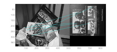

my implementation gives me a very bad matching. alot more work to do.

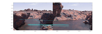
and more bad results, if the orientation of the keypoint is wrong, the matching will also suffer so i tired different tangents in matlab

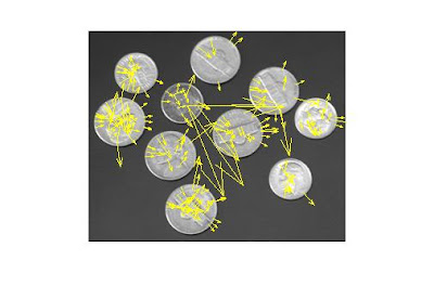
atan(dy/dx);

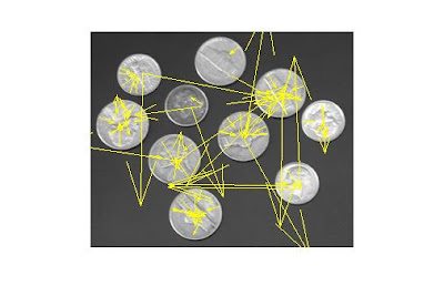
atan2(dy,dx);

BOTH IMAGES: show clearly that rotation invariance is not achieved, this is the reason why the matching gives alot of false negative results

furthermore; the amount of BLUR is also very important

images and details from (based on my understanding):
Lowe, David G. “Distinctive Image Features from Scale­ Invariant Keypoints”. International Journal of Computer Vision, 60, 2 (2004)

My SIFT implementation and comparisons

Im trying to implement SIFT in matlab and compare it with other implementations
the comparisons are against the following:
original SIFT code by LOWE found at this URL
the other is the popular A. Vedaldi Code found at this URL


This is the result of the vadaldi code that finds 262 key points

This is the original SIFT code by David Lowe showing 249 keypoints



This is from my code showing 315 keypoints.

from all 3 images you can see that there are points that are outside of the image and a surprising 70 extra keypoints on my implementation. obviously my implementation is wrong, so i tried to go through the code and adjusted a few things

Now i get 195 keypoints and as you can see from the image, all the keypoints are located inside of the image. my next problem is the magnitude.

from the previous images, the code from LOWE and VEDALDI have a very good magnitude however my implementation has very small.




All yellow markers are from my implementation

Computer vision Datasets to use

a very nice dataset collected by Krystian Mikolajczyk for testing scaled and affine interest point detectors with various types of local image descriptors.
These are some of the other dataset that i use:

MIT Face Dataset
MIT Car Datasets
MIT Street Scenes
Pedestrian dataset from MIT

Most of the files are in *.ppm format, i personally use adobe photoshop to open these

background subtraction (problems)

there are several problems that must
be addressed by a good background removal algorithm to
correctly detect moving objects. A good background removal
algorithm should handle the relocation of background objects,
non-stationary background objects e.g. waving trees,
and image changes due to camera motion which is common
in outdoor applications e.g. wind load. A background removal
system should adapt to illumination changes whether
gradual changes (time of day) or sudden changes (lightswitch),
whether global or local changes such as shadows and interreflections.
A foreground object might have similar characteristics
as the background, it become difficult to distinguish
between them (camouflage). A foreground object that becomes
motionless can not be distinguished from a background
object that moves and then becomes motionless
(sleeping person). A common problem faced in the background
initialization phase is the existence of foreground
objects in the training period, which occlude the actual background,
and on the other hand often it is impossible to clear
an area to get a clear view of the background, this puts serious
limitations on system to be used in high traffic areas.
Some of these problems can be handled by very computationally
expensive methods, but in many applications, a short
processing time is required.

for a few see the following: POST1 - POST2 - POST3

Image Filtering (Gaussian)

A filter is any kind of processing that has one characteristic: it takes a signal as the input and produces a relevant output signal after processing it in some way. A filter can always be mathematically described.

An example of a 1D filter:

1 2 3 4 3 2 1

An example of a 2D filter:

1 1 1 1 1
1 2 2 2 1
1 2 3 2 1
1 2 2 2 1
1 1 1 1 1

A 2D filter as well as the 1D filter, has to have an odd number of samples in both the vertical as well as the horizontal orientation.

In Matlab:
n represents the number of cells so for a 2D 3x3 filter n=9 for a 1D filter the number of cells in my example above is 7


% 2D Gaussian Filter
x = -1/2:1/(n-1):1/2;
[Y,X] = meshgrid(x,x);
f = exp( -(X.ˆ2+Y.ˆ2)/(2*sˆ2) );
f = f / sum(f(:));



%1D Gaussian Filter
x = -1/2:1/(n-1):1/2;
f = exp( -(x.^2)/(2*sigma^2) );
g = f / sum(sum(f));

Object detection Problem

one of the main problems of object tracking is identifying the object to be tracked. from my previous POST, i selected the object manually

Object detection is a necessary step for any tracking algorithm because the algorithm needs to identify the moving object. The objective of object detection is to find out the position of the object and the region it occupies in the first frame.

This task is extremely difficult due to the complex shapes of the moving targets. In order to simplify the problem, a variety of constrains are imposed to help in finding the object in image plane, such as the number of objects to be tracked, types of objects, etc. Currently, there are three popular techniques used in object tracking: image segmentation, background subtraction and supervised learning algorithms.

PROBLEMS
background subtraction is used for fixed cameras for moving camera we can use SIFT to stabilize the camera and perform background subtraction. However we do not get 100% stability with this method.
The image segmentation methods are able to partition the image into perceptually similar regions, but the criteria for a good partition and the efficiency are two problems that the image segmentation algorithms need to address.

The main drawback for supervised learning methods is that they usually require a large collection of samples from each object class and the samples must be manually labeled.


SOURCE : Tracking of Multiple Objects under Partial Occlusion - Bing Han, Christopher Paulson, Taoran Lu, Dapeng Wu, Jian Li - 2010

SIFT tracking set1

Video: Result of identification for tracking


the objective is to find an object in the foreground place a rectangle around the object and find SIFT keypoints in that rectangle, for the next frames only match those keypoints from the rectangle to the image

images and details from (based on my understanding):
Lowe, David G. “Distinctive Image Features from Scale­ Invariant Keypoints”. International Journal of Computer Vision, 60, 2 (2004)

The STEPS:

1. go through all the video and find SIFT keypoints in each frame
2. from an initial frame, select a moving object or foreground and place a rectangle around it
3. get all the SIFT keypoints in that rectangle
4. match the points from that rectangle to all the other points found in step 1
5. if match is found place a rectangle in succeeding frames

problem: in some frames keypoints dont match,thats the reason why i loose track of the vehicle
its either there arent enough matches or those keypoints are different from the first frame
again i consider the keypoints found only in the first frame and compare to new frames

TO DO: compare points from first frame to the next.if object found get the new SIFT points of that object from the new frame and then compare to succeeding frame.

objective: track using SIFT points without needed to preselect the cars

code:

img = imread([imgDir '\' fileNames(3).name]);
[r c bands] = size(img);
h=figure;
imshow(img);
hold on;

....

title('Click the top left corner of an object to track...');
[x1 y1] = ginput(1);
plot(x1, y1, 'rx');
title(sprintf('Click the bottom right corner (Right click indicates last object)'));
[x2 y2 button] = ginput(1);
objectCount = objectCount+1;
rectangle('Position', [x1 y1 x2-x1 y2-y1], 'LineWidth', 4, 'EdgeColor', colors(mod(objectCount, size(colors,1))+1, :));

.....

% Find the sift features for the object
imwrite(trackingObjects{objectCount}.img, 'tmp.pgm', 'pgm');
[jnk des locs] = sift('tmp.pgm');
trackingObjects{objectCount}.des = des;

....

% Read in the next image
img = imread([imgDir '\' fileNames(ii).name]);

% Show the image
figure(h)
cla;
imshow(img); hold on;

% Look for features in the image for each object we are tracking

.....

% Match the features for this object
clear match;
match = matchFeatures(trackingObjects{jj}.des, des);
clear newLocs
newLocs = locs(match(match>0), :);

% Only proceed if we found at least one match
if ~isempty(newLocs)
print('match ound');
....

SIFT by lowe using ImageJ (PARTIAL)

create a a plain text file and place the code in it.
from within ImageJ, open any image
From the ImageJ menu select PLUGINS -> MACRO's -> RUN

results show the first 2 steps of SIFT, however the 3 step takes alot of time to process because we are going through each pixel and thats done for all 4 octaves.

for short overview of SIFT please see my post HERE

//*************************************************

// SIFT Step 1: Constructing a scale space

//*************************************************
//Lowe claims blur the image with a sigma of 0.5 and double it's dimensions

width=getWidth(); height=getHeight();

//------------------------------------------------------------------------
// convert to 8-bit gray scale and create scale space for the first octave
//------------------------------------------------------------------------

run("Duplicate...", "title=[Copy of original]");
Oid = getImageID;
run("8-bit");

run("Duplicate...", "title=[Octave 1 blur1]");
P1id1 = getImageID;
run("Gaussian Blur...", "slice radius=2"); //blur 1

run("Duplicate...", "title=[Octave 1 blur 2]");
P1id2 = getImageID;
run("Gaussian Blur...", "slice radius=4"); //blur 2

run("Duplicate...", "title=[Octave 1 blur 3]");
P1id3 = getImageID;
run("Gaussian Blur...", "slice radius=8"); //blur 3

run("Duplicate...", "title=[Octave 1 blur 4]");
P1id4 = getImageID;
run("Gaussian Blur...", "slice radius=16"); //blur 4

run("Duplicate...", "title=[Octave 1 blur 5]");
P1id5 = getImageID;
run("Gaussian Blur...", "slice radius=16"); //blur 5
showMessage("DONE", "First OCTAVE");
//----------------------------------------------------------------------------
// Perform image resize on original and create second octave
//----------------------------------------------------------------------------

selectImage(Oid);
run("Size...", "width="+width/2+" height="+ height/2);
run("Duplicate...", "title=[Octave 2 blur1]"); P2id1 = getImageID; run("Gaussian Blur...", "slice radius=2"); //blur 1
run("Duplicate...", "title=[Octave 2 blur 2]"); P2id2 = getImageID; run("Gaussian Blur...", "slice radius=4"); //blur 2
run("Duplicate...", "title=[Octave 2 blur 3]"); P2id3 = getImageID; run("Gaussian Blur...", "slice radius=8"); //blur 3
run("Duplicate...", "title=[Octave 2 blur 4]"); P2id4 = getImageID; run("Gaussian Blur...", "slice radius=16"); //blur 4
run("Duplicate...", "title=[Octave 2 blur 5]"); P2id5 = getImageID; run("Gaussian Blur...", "slice radius=16"); //blur 5

showMessage("DONE", "Second OCTAVE");

//----------------------------------------------------------------------------
// Perform image resize on original and create Third octave
//----------------------------------------------------------------------------

selectImage(Oid);
run("Size...", "width="+width/4+" height="+ height/4);
run("Duplicate...", "title=[Octave 3 blur1]"); P3id1 = getImageID; run("Gaussian Blur...", "slice radius=2"); //blur 1
run("Duplicate...", "title=[Octave 3 blur 2]"); P3id2 = getImageID; run("Gaussian Blur...", "slice radius=4"); //blur 2
run("Duplicate...", "title=[Octave 3 blur 3]"); P3id3 = getImageID; run("Gaussian Blur...", "slice radius=8"); //blur 3
run("Duplicate...", "title=[Octave 3 blur 4]"); P3id4 = getImageID; run("Gaussian Blur...", "slice radius=16"); //blur 4
run("Duplicate...", "title=[Octave 3 blur 5]"); P3id5 = getImageID; run("Gaussian Blur...", "slice radius=16"); //blur 5
showMessage("DONE", "Third OCTAVE");

//------------------------------------------------------------------------------
// Perform image resize on original and create Forth octave
//------------------------------------------------------------------------------

selectImage(Oid);
run("Size...", "width="+width/8+" height="+ height/8);

run("Duplicate...", "title=[Octave 4 blur1]"); P4id1 = getImageID; run("Gaussian Blur...", "slice radius=2"); //blur 1
run("Duplicate...", "title=[Octave 4 blur 2]"); P4id2 = getImageID; run("Gaussian Blur...", "slice radius=4"); //blur 2
run("Duplicate...", "title=[Octave 4 blur 3]"); P4id3 = getImageID; run("Gaussian Blur...", "slice radius=8"); //blur 3
run("Duplicate...", "title=[Octave 4 blur 4]"); P4id4 = getImageID; run("Gaussian Blur...", "slice radius=16"); //blur 4
run("Duplicate...", "title=[Octave 4 blur 5]"); P4id5 = getImageID; run("Gaussian Blur...", "slice radius=16"); //blur 5

showMessage("DONE", "Forth OCTAVE");

//**********************************************************
// SIFT Step 2: Laplacian of Gaussian Approximation
//**********************************************************

// input is 5 blurred images per octave
// output is 4 images per octave

imageCalculator('subtract', P1id1, P1id2); Q1I1 = getImageID; rename("Result Subtract Octave 1");
imageCalculator('subtract', P1id2, P1id3); Q1I2 = getImageID; rename("Result Subtract Octave 1");
imageCalculator('subtract', P1id3, P1id4); Q1I3 = getImageID; rename("Result Subtract Octave 1");
imageCalculator('subtract', P1id4, P1id5); Q1I4 = getImageID; rename("Result Subtract Octave 1");

imageCalculator('subtract', P2id1, P2id2); Q2I1 = getImageID; rename("Result Subtract Octave 2");
imageCalculator('subtract', P2id2, P2id3); Q2I2 = getImageID; rename("Result Subtract Octave 2");
imageCalculator('subtract', P2id3, P2id4); Q2I3 = getImageID; rename("Result Subtract Octave 2");
imageCalculator('subtract', P2id4, P2id5); Q2I4 = getImageID; rename("Result Subtract Octave 2");

imageCalculator('subtract', P3id1, P3id2); Q3I1 = getImageID; rename("Result Subtract Octave 3");
imageCalculator('subtract', P3id2, P3id3); Q3I2 = getImageID; rename("Result Subtract Octave 3");
imageCalculator('subtract', P3id3, P3id4); Q3I3 = getImageID; rename("Result Subtract Octave 3");
imageCalculator('subtract', P3id4, P3id5); Q3I4 = getImageID; rename("Result Subtract Octave 3");

imageCalculator('subtract', P3id1, P3id2); Q4I1 = getImageID; rename("Result Subtract Octave 4");
imageCalculator('subtract', P3id2, P3id3); Q4I2 = getImageID; rename("Result Subtract Octave 4");
imageCalculator('subtract', P3id3, P3id4); Q4I3 = getImageID; rename("Result Subtract Octave 4");
imageCalculator('subtract', P3id4, P3id5); Q4I4 = getImageID; rename("Result Subtract Octave 4");

//************************************************************
// SIFT Step 3: Finding key points
//************************************************************

//need to generate 2 extrema images
// maxima and minima almost never lies exactly on a pixel. since its between pixels we need to locate it mathematically using Tylor expansion


//--------------------------------------------------------------------------------
// first octave
//--------------------------------------------------------------------------------


/*
selectImage(Q1I2);
width=getWidth(); height=getHeight();

num = 0; //number of points
numRemoved = 0; //failed tested points

for (xi=1; xi<width; xi++)
{
for(yi=1; yi<height; yi++)
{
justSet = 1;
currentPixel = getPixel(xi, yi);

if ( (currentPixel > getPixel(yi+1, xi)) &
(currentPixel > getPixel(yi+1, xi) ) &
(currentPixel > getPixel(yi, xi-1) ) &
(currentPixel > getPixel(yi, xi+1)) &
(currentPixel > getPixel(yi-1, xi-1) ) &
(currentPixel > getPixel(yi-1, xi+1) ) &
(currentPixel > getPixel(yi+1, xi+1) ) &
(currentPixel > getPixel(yi+1, xi-1)) )
{

selectImage(Q1I1);
if ( (currentPixel > getPixel(yi+1, xi)) &
(currentPixel > getPixel(yi+1, xi) ) &
(currentPixel > getPixel(yi, xi-1) ) &
(currentPixel > getPixel(yi, xi+1)) &
(currentPixel > getPixel(yi-1, xi-1) ) &
(currentPixel > getPixel(yi-1, xi+1) ) &
(currentPixel > getPixel(yi+1, xi+1) ) &
(currentPixel > getPixel(yi+1, xi-1)) )

{
selectImage(Q1I3);
if ( (currentPixel > getPixel(yi+1, xi)) &
(currentPixel > getPixel(yi+1, xi) ) &
(currentPixel > getPixel(yi, xi-1) ) &
(currentPixel > getPixel(yi, xi+1)) &
(currentPixel > getPixel(yi-1, xi-1) ) &
(currentPixel > getPixel(yi-1, xi+1) ) &
(currentPixel > getPixel(yi+1, xi+1) ) &
(currentPixel > getPixel(yi+1, xi-1)) )

{
num++;
}
}

}
}
}
print("first part= " + num);

selectImage(Q1I3);
width=getWidth(); height=getHeight();
for (xi=1; xi<width; xi++)
{
for(yi=1; yi<height; yi++)
{
justSet = 1;
currentPixel = getPixel(xi, yi);

if ( (currentPixel > getPixel(yi+1, xi)) &
(currentPixel > getPixel(yi+1, xi) ) &
(currentPixel > getPixel(yi, xi-1) ) &
(currentPixel > getPixel(yi, xi+1)) &
(currentPixel > getPixel(yi-1, xi-1) ) &
(currentPixel > getPixel(yi-1, xi+1) ) &
(currentPixel > getPixel(yi+1, xi+1) ) &
(currentPixel > getPixel(yi+1, xi-1)) )
{

selectImage(Q1I2);
if ( (currentPixel > getPixel(yi+1, xi)) &
(currentPixel > getPixel(yi+1, xi) ) &
(currentPixel > getPixel(yi, xi-1) ) &
(currentPixel > getPixel(yi, xi+1)) &
(currentPixel > getPixel(yi-1, xi-1) ) &
(currentPixel > getPixel(yi-1, xi+1) ) &
(currentPixel > getPixel(yi+1, xi+1) ) &
(currentPixel > getPixel(yi+1, xi-1)) )

{

selectImage(Q1I4);
if ( (currentPixel > getPixel(yi+1, xi)) &
(currentPixel > getPixel(yi+1, xi) ) &
(currentPixel > getPixel(yi, xi-1) ) &
(currentPixel > getPixel(yi, xi+1)) &
(currentPixel > getPixel(yi-1, xi-1) ) &
(currentPixel > getPixel(yi-1, xi+1) ) &
(currentPixel > getPixel(yi+1, xi+1) ) &
(currentPixel > getPixel(yi+1, xi-1)) )

{

num++;

}
}

}
}
}
print("second part= "+num);

*/


//+++++++++++++++++++++++++++++++++++++++++++
// process takes too long... alternative MY IDEA

//+++++++++++++++++++++++++++++++++++++++++++

Randomly select points and compare it to a threshold if its maximum or minimum to the 26 neighbors then consider that point to be on a blob based on:

T. Lindeberg. Scale-Space Theory in Computer Vision.
Kluwer Academic Publishers, Norwell, MA, USA, 1994.
Quote: "local extrema points are located in a blob region"

So instead of going through each pixel of the image in multiple scales: select a specific number of random points and compare with the 26 neighbors. if you get a specific number of points that are maximum of minimum then continue to the next step if not get another set of random points until your specific number of maximum and minimum points are found.

CODE TO FOLLOW

Angled stereo vision

The distance between the lenses in a typical stereo camera (the intra-axial distance) is about the distance between one's eyes (known as the intra-ocular distance) and is about 6.35cm, though a longer base line (greater inter-camera distance) produces more extreme 3-dimensionality.

However we have 2 cameras which are angled in contrast to the stereo vision camera where both cameras are parallel on a line

Hessian Matrix

In mathematics, the Hessian matrix (or simply the Hessian) is the square matrix of second-order partial derivatives of a function; that is, it describes the local curvature of a function of many variables. The second derivative can be applied at a non-degenerate critical point x. If the Hessian is positive definite at x, then f attains a local minimum at x. If the Hessian is negative definite at x, then f attains a local maximum at x. If the Hessian has both positive and negative eigenvalues then x is a saddle point for f (this is true even if x is degenerate). Otherwise the test is inconclusive. In view of what has just been said, the second derivative test for functions of one and two variables is simple. In one variable, the Hessian contains just one second derivative; if it is positive then x is a local minimum, if it is negative then x is a local maximum; if it is zero then the test is inconclusive. In two variables, the discriminant can be used, because the determinant is the product of the eigenvalues. If it is positive then the eigenvalues are both positive, or both negative. If it is negative then the two eigenvalues have different signs. If it is zero, then the second derivative test is inconclusive(wikipdia).

consider a continuous function of two variables such that the value of the function at (x,y) is given by f(x,y). The Hessian matrix, H, is the matrix of partial derivates of the function f.



The determinant of this matrix, known as the discriminant, is calculated by:


The value of the discriminant is used to classify the maxima and minima of the function by the second order derivative test. Since the determinant is the product of eigenvalues of the Hessian we can classify the points based on the sign of the result. If the determinant is negative then the eigenvalues have different signs and hence the point is not a local extremum; if it is positive then either both eigenvalues are positive or both are negative and in either case the point is classified as an extremum.

NOTE:

We can calculate the derivatives by convolution with an appropriate kernel. In the case of SURF the second order scale normalised Gaussian is the chosen filter as it allows for analysis over scales as well as space. We can construct kernels for the Gaussian derivatives in x, y and combined xy direction such that we calculate the four entries of the Hessian matrix. Use of the Gaussian allows us to vary the amount of smoothing during the convolution stage so that the determinant is calculated at different scales. Furthermore, since the Gaussian is an isotropic (i.e. circularly symmetric) function, convolution with the kernel allows for rotation invariance.

Lowe found performance increase in approximating the Laplacian of Gaussians by a difference of Gaussians. In a similiar manner, Bay proposed an approximation to the Laplacian of Gaussians by using box filter representations of the respective kernels.

Histogram

A histogram is one of the basic quality tools. It is used to graphically summarize and display the distribution and variation of a process data set. A frequency distribution shows how often each different value in a set of data occurs. The main purpose of a histogram is to clarify the presentation of data.

• • •
What is the most common system response?
What distribution (center, variation and shape) does the data have?
Does the data look symmetric or is it skewed to the left or right?

Typical applications of histograms in root cause analysis include:
• Presenting data to determine which causes dominate
• Understanding the distribution of occurrences of different problems, causes,consequences, etc.

Weaknesses
There are two weaknesses of histograms that you should bear in mind. The first is that histograms can be manipulated to show different pictures. If too few or too many bars are used, the histogram can be misleading. This is an area which requires some judgment, and perhaps some experimentation, based on the analyst's experience.
Histograms can also obscure the time differences among data sets.
furthermore there is a loss of individual measurements due to grouping. Misrepresentation of data from groups that are too wide or too narrow.

Distributions to encounter:

Bi-Modal (double-peaked)
Distribution appears to have two peaks
• May indicate that data from more than one process are mixed together
o Materials may have come from two separate vendors
o Samples may have come from two separate machines
• A bi-modal curve often means that the data actually reflects two distinct processes with different centers. You will need to distinguish between the two processes to get a clear view of what is really happening in either individual process.

SURF Details (Speed Up Robust Features)

SURF (Speeded Up Robust Features) is a robust image detector & descriptor, first presented by Herbert Bay et al. in 2006, that can be used in computer vision tasks like object recognition or 3D reconstruction. It is partly inspired by the SIFT descriptor. The standard version of SURF is several times faster than SIFT and claimed by its authors to be more robust against different image transformations than SIFT. SURF is based on sums of approximated 2D Haar wavelet responses and makes an efficient use of integral images. As basic image features it uses a Haar wavelet approximation of the determinant of Hessian blob detector (WIKIPEDIA).

The performance gain in the SURF Implementation is due to use of integral images (See my post on Integral Images)

In constructing the scale space, Lowe proposed a difference of Gaussian to approximate the Laplacian of Gaussian.The images were blurred and subsampled to produce a scale space. After which the difference of gaussian was used to estimate the laplacian gaussian.

in SURF this was done using a box filter representation of a kernel. This kernel was used to produce the pyramid and kept the original image unchanged while changing the filter size.

TO DO: Add more of the details

PCA-SIFT Details

PCA-SIFT was introduced as an improvement for SIFT. The implementation only differs in the 4th step (keypoint descriptor). PCA-SIFT uses Principal Component Analysis (PCA) instead of a histogram to normalize the gradient patch. Hence, the feature vector is significantly smaller than the standard SIFT feature vector.

It differs from the original SIFT implementation in its forth stage. By reducing the 128 element of the original SIFT using PCA, results in a significant space benefit.

Another difference is the input vector is created by concatenating the horizontal and vertical gradient maps for 41x41 patch centered at the keypoint. Producing 2x39x39 = 3042 vector elements. The fewer components of PCA-SIFT requires less storage therefore, resulting in faster matching. The dimensionality of this feature space is arbitrary chosen as n=20, which results in a significant space benefit.

TO DO: add more detail

The Log-Polar Transform

The log-polar transform is a simple operation that changes the coordinate system of an image from Cartesian to log-polar.

Before and after conversion to logpolar coordinate system

Log-polar coordinates have several interesting properties::..
First, when optical flow is computed as the camera moves along the optical axis (as is common in robotics), the optical flow vectors are radial from the image center. However, in log-polar coordinates, the flow vectors are vertical. This can make the detection of moving objects more efficient computationally.

Second, the log polar transform converts an image to a form that is rotation and scale invariant. This can be very helpful for object detection. Finally, the log-polar transform emulates how images appear on the back of the human retina. (The brain then transforms the image to the Cartesian-like way we perceive it.)

In Matlab (http://www.mathworks.com/matlabcentral/newsreader/view_thread/108599):

function [pim,zoff] = PolarTransform(img,zcenter,rs,thetas)
% function [pim,zoff] = PolarTransform(img,zcenter,rs,thetas)
% extract the polar transform of a section of img
% polar transform origin at zcenter(x+iy)
% rs(pixels),thetas(radians) are sets of radii and angles to sample
% if they are scalars, then the radii are 1:r
% and thetas is taken to be dtheta in
% thetas = linspace(0, 2*pi , round(2*pi/dtheta) ); thetas =
thetas(1:end-1)
% zoff are the coordinates of the sample points in the original image
(x+iy)
% REA 4/15-6/1/05
if isscalar(rs)
rs = 1:round(rs);
end

if isscalar(thetas)
thetas = linspace(0, 2*pi , round(2*pi/thetas) );
thetas = thetas(1: (end-1) );
end

[thetas_img,rs_img] = meshgrid(thetas,rs);
[xs,ys] = pol2cart(thetas_img,rs_img);

% offset the x,y coords to the appropriate location
zoff = complex(xs,ys) + zcenter;

% and extract the image data
pim = interp2(img,real(zoff),imag(zoff),'nearest');

Furthermore:

Cartesian Coordinate System Conversion

cart2pol	Transform Cartesian coordinates to polar or cylindrical
cart2sph	Transform Cartesian coordinates to spherical
pol2cart	Transform polar or cylindrical coordinates to Cartesian
sph2cart	Transform spherical coordinates to Cartesian