Pyramids

It is a type of multi-scale signal representation developed by the computer vision, image processing and signal processing communities, in which a signal or an image is subject to repeated smoothing and subsampling. Historically, pyramid representation is a predecessor to scale space representation and multiresolution analysis (WIKIPEDIA).

There are 2 types of pyramids: the lowpass and bandpass.
SIFT uses LOWPASS pyramids: A lowpass pyramid is generated by first smoothing the image with an appropriate smoothing filter and then subsampling the smoothed image, usually by a factor of two along each coordinate direction.



A bandpass pyramid is obtained by forming the difference between adjacent levels in a pyramid, where in addition some kind of interpolation is performed between representations at adjacent levels of resolution, to enable the computation of pixelwise differences.

Disadvantage:
Pyramid representation leads to rapidly decreasing image size. This reduces computational work in computation of the representation and subsequent processing. The main disadvantage of with pyramids is that they are defined from a logarithmic process, making theoritical analysis complicated. Furthermore, they correspond to quite a coarse quantization along the scale direction, which makes logarithmically hard to relate images structures across multiple scales. ...


A scale-space is a continuous function which can be used to find extrema across all possible scales [A. Witkin. Scale-space filtering, int. joint conf. Artif. Intell, 2:1019–1021, 1983.].

In computer vision the scale-space is typically implemented as an image pyramid where the input image is iteratively convolved with Gaussian kernel and repeatedly sub-sampled (reduced in size). This method is used to great effect in SIFT (See my post of SIFT Details) but since each layer relies on the previous, and images need to be resized it is not computationally efficient.

Another way to construct the scale-space is by applying kernels of increasing size to the original image. This allows for multiple layers of the scale-space pyramid to be processed simultaneously and negates the need to subsample the image hence providing performance increase.

The SURF approach leaves the original image unchanged and varies only the filter size.

References:

H. Bay, T. Tuytelaars, and L. Van Gool. Surf: Speeded up robust features. European Conference on Computer Vision, 1:404–417, 2006.

D.G. Lowe. Distinctive image features from scale-invariant keypoints. International Journal of Computer Vision, 60(2):91–110, 2004.

Standard deviation Map or Image variance

The implementation calculates the variance of neighboring pixels given a window around a center pixel.

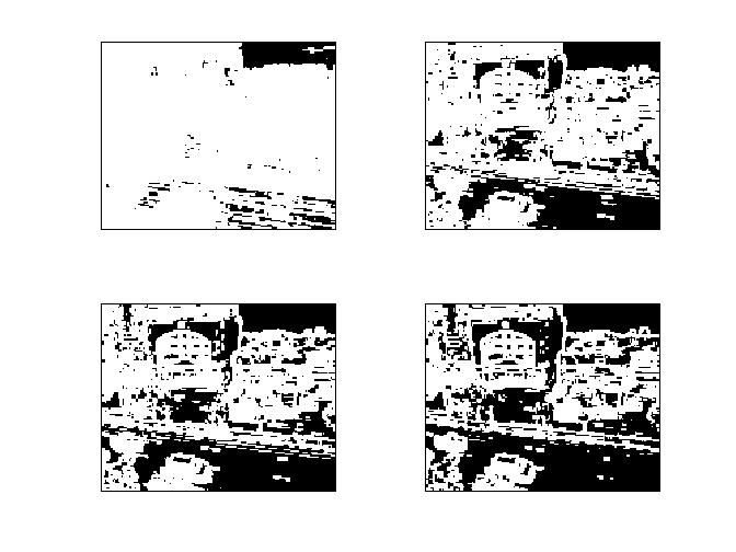
ive used a window size of 3. this means i have a square window of 3x3. the image ive used if the following:



This is the result. ive tried to vary the threshold to get different results. in the bottom image. starting from the top left to right ive used a threshold of 10, 100, 160, 200. The results are very similar to to an adaptive threshold with the exception of it being a negative image. you can see my results on adaptive threshold HERE>>>

Take note that variance is computed for a single image. Just like Background subtraction, it is very sensitive to the threshold and may require trial and error to get good result. however on a cluttered image, it seems very irrational to use this method to identify objects.

I used the same method on a single object on the screen. and i get different results by varying the threshold. Over all it can identify the object very clearly. although setting the right threshold requires alot of trial and error. In the end it has some noise which needs to be removed in the end using morphology.

Meanshift Tracking algorithm

Mean shift

The main function of this algorithm is histogram estimation. Since moving objects can be identified by their color histogram. Mean-shift tracking algorithm is an iterative scheme based on comparing the histogram of the original object in the current image frame and histogram of candidate regions in the next image frame. The aim is to maximize the correlation between two histograms.

Code:


Mv = aviread('StabilizationResult.avi')
rmin = 0; %min row value for search window
rmax = 0; %max row value for search window
cmin = 0; %min col value for search window
cmax = 0; %max col value for search window
numofframes = 0;
frameNo = 10; %starting frame
vidSize=[128 160]; %video size
centerold = [0 0];
centernew = [0 0];

M =Mv;

% get number of frames
numberofframes = length(M);

Frame1 = M(frameNo);
Image1 = imresize(Frame1.cdata,vidSize,'bilinear');
disp('Click and drag mouse for an initial box window');
% get search window for first frame
[ cmin, cmax, rmin, rmax ] = select( Image1 );
cmin = round(cmin);
cmax = round(cmax);
rmin = round(rmin);
rmax = round(rmax);
wsize(1) = abs(rmax - rmin);
wsize(2) = abs(cmax - cmin);

hue=Image1(:,:,1);
histogram = zeros(256);

for i=rmin:rmax
for j=cmin:cmax
index = uint8(hue(i,j)+1);
%count number of each pixel
histogram(index) = histogram(index) + 1;
end
end

% for each frame
for i = frameNo:numberofframes
Frame = M(i);
I = imresize(Frame.cdata,vidSize,'bilinear');

hue= I(:,:,1);
[rows cols] = size(hue);
probmap = zeros(rows, cols);
for r=1:rows
for c=1:cols
if(hue(r,c) ~= 0)
probmap(r,c)= histogram(hue(r,c));
end
end
end
probmap = probmap/max(max(probmap));
probmap = probmap*255;

count = 0;

rowcenter = 0; % any number just so it runs through at least twice
colcenter = 0;
rowcenterold = 30;
colcenterold = 30;
while (((abs(rowcenter - rowcenterold) > 2) && (abs(colcenter - colcenterold) > 2)) || (count < 15) )
rowcenterold = rowcenter;
colcenterold = colcenter;

[ rowcenter colcenter M00 ] = meanshift(rmin, rmax, cmin,...
cmax, probmap);

rmin = round(rowcenter - wsize(1)/2);
if rmin<1 br=""> rmin=1;
end
rmax = round(rowcenter + wsize(1)/2);
if rmax<1 br=""> rmax=1;
end
cmin = round(colcenter - wsize(2)/2);
if cmin<1 br=""> cmin=1;
end
cmax = round(colcenter + wsize(2)/2);
if cmax<1 br=""> cmax=1;
end
wsize(1) = abs(rmax - rmin);
wsize(2) = abs(cmax - cmin);

count = count + 1;
end

G = I;
trackim=G;

%make box of current search window on saved image
for r= rmin:rmax
trackim(r, cmin:cmin+2) = 0;
trackim(r, cmax-2:cmax) = 0;
end
for c= cmin:cmax
trackim(rmin:rmin+2, c) = 0;
trackim(rmax-2:rmax, c) = 0;
end

windowsize = 100 * (M00/256)^.5;
sidelength = sqrt(windowsize);
rmin = round(rowcenter-sidelength/2);
if rmin<1 br=""> rmin=1;
end
rmax = round(rowcenter+sidelength/2);
if rmax<1 br=""> rmax=1;
end
cmin = round(colcenter-sidelength/2);
if cmin<1 br=""> cmin=1;
end
cmax = round(colcenter+sidelength/2);
if cmax<1 br=""> cmax=1;
end
wsize(1) = abs(rmax - rmin);
wsize(2) = abs(cmax - cmin);


outname = sprintf('./answer/%d.jpg', i);
imwrite(trackim, outname);

figure(1),imshow(trackim); hold on
end
hold off;

Tracking using Optical Flow

Optical flow with Hierarchical Lucas Kanade (using pyramids)

results are very strange!














Horn’s optical flow algorithm. Results are unclear.




Code:

function [u,v,cert] = HierarchicalLK(im1, im2, numLevels, windowSize, iterations, display)
%HIERARCHICALLK Hierarchical Lucas Kanade (using pyramids)
% [u,v]=HierarchicalLK(im1, im2, numLevels, windowSize, iterations, display)

if (size(im1,1)~=size(im2,1)) | (size(im1,2)~=size(im2,2))
error('images are not same size');
end;

if (size(im1,3) ~= 1) | (size(im2, 3) ~= 1)
error('input should be gray level images');
end;


% check image sizes and crop if not divisible
if (rem(size(im1,1), 2^(numLevels - 1)) ~= 0)
warning('image will be cropped in height, size of output will be smaller than input!');
im1 = im1(1:(size(im1,1) - rem(size(im1,1), 2^(numLevels - 1))), :);
im2 = im2(1:(size(im1,1) - rem(size(im1,1), 2^(numLevels - 1))), :);
end;

if (rem(size(im1,2), 2^(numLevels - 1)) ~= 0)
warning('image will be cropped in width, size of output will be smaller than input!');
im1 = im1(:, 1:(size(im1,2) - rem(size(im1,2), 2^(numLevels - 1))));
im2 = im2(:, 1:(size(im1,2) - rem(size(im1,2), 2^(numLevels - 1))));
end;

%Build Pyramids
pyramid1 = im1;
pyramid2 = im2;

for i=2:numLevels
im1 = reduce(im1);
im2 = reduce(im2);
pyramid1(1:size(im1,1), 1:size(im1,2), i) = im1;
pyramid2(1:size(im2,1), 1:size(im2,2), i) = im2;
end;

% base level computation
disp('Computing Level 1');
baseIm1 = pyramid1(1:(size(pyramid1,1)/(2^(numLevels-1))), 1:(size(pyramid1,2)/(2^(numLevels-1))), numLevels);
baseIm2 = pyramid2(1:(size(pyramid2,1)/(2^(numLevels-1))), 1:(size(pyramid2,2)/(2^(numLevels-1))), numLevels);
[u,v] = LucasKanade(baseIm1, baseIm2, windowSize);

for r = 1:iterations
[u, v] = LucasKanadeRefined(u, v, baseIm1, baseIm2);
end

%propagating flow 2 higher levels
for i = 2:numLevels
disp(['Computing Level ', num2str(i)]);
uEx = 2 * imresize(u,size(u)*2); % use appropriate expand function (gaussian, bilinear, cubic, etc).
vEx = 2 * imresize(v,size(v)*2);

curIm1 = pyramid1(1:(size(pyramid1,1)/(2^(numLevels - i))), 1:(size(pyramid1,2)/(2^(numLevels - i))), (numLevels - i)+1);
curIm2 = pyramid2(1:(size(pyramid2,1)/(2^(numLevels - i))), 1:(size(pyramid2,2)/(2^(numLevels - i))), (numLevels - i)+1);

[u, v] = LucasKanadeRefined(uEx, vEx, curIm1, curIm2);

for r = 1:iterations
[u, v, cert] = LucasKanadeRefined(u, v, curIm1, curIm2);
end
end;

if (display==1)
figure, quiver(reduce((reduce(medfilt2(flipud(u),[5 5])))), -reduce((reduce(medfilt2(flipud(v),[5 5])))), 0), axis equal
end


Code:

%Implementation based on Horn’s optical flow algorithm.
function [u, v] = LucasKanade(im1, im2, windowSize);
%LucasKanade lucas kanade algorithm, without pyramids (only 1 level);

%REVISION: NaN vals are replaced by zeros

[fx, fy, ft] = ComputeDerivatives(im1, im2);

u = zeros(size(im1));
v = zeros(size(im2));

halfWindow = floor(windowSize/2);
for i = halfWindow+1:size(fx,1)-halfWindow
for j = halfWindow+1:size(fx,2)-halfWindow
curFx = fx(i-halfWindow:i+halfWindow, j-halfWindow:j+halfWindow);
curFy = fy(i-halfWindow:i+halfWindow, j-halfWindow:j+halfWindow);
curFt = ft(i-halfWindow:i+halfWindow, j-halfWindow:j+halfWindow);

curFx = curFx';
curFy = curFy';
curFt = curFt';


curFx = curFx(:);
curFy = curFy(:);
curFt = -curFt(:);

A = [curFx curFy];

U = pinv(A'*A)*A'*curFt;

u(i,j)=U(1);
v(i,j)=U(2);
end;
end;

u(isnan(u))=0;
v(isnan(v))=0;

%u=u(2:size(u,1), 2:size(u,2));
%v=v(2:size(v,1), 2:size(v,2));

%%%%%%%%%%%%%%%%%%%%%%%%%%%%%%%%%%%%%%%%%%%%%%%%%%%%%%%%%%%%%%%%%%%%%%%%%%%%%
function [fx, fy, ft] = ComputeDerivatives(im1, im2);
%ComputeDerivatives Compute horizontal, vertical and time derivative
% between two gray-level images.

if (size(im1,1) ~= size(im2,1)) | (size(im1,2) ~= size(im2,2))
error('input images are not the same size');
end;

if (size(im1,3)~=1) | (size(im2,3)~=1)
error('method only works for gray-level images');
end;


fx = conv2(double(im1),double(0.25* [-1 1; -1 1])) + conv2(double(im2), double(0.25*[-1 1; -1 1]));
fy = conv2(double(im1), double(0.25*[-1 -1; 1 1])) + conv2(double(im2), double(0.25*[-1 -1; 1 1]));
ft = conv2(double(im1), double(0.25*ones(2))) + conv2(double(im2),double( -0.25*ones(2)));

% make same size as input
fx=fx(1:size(fx,1)-1, 1:size(fx,2)-1);
fy=fy(1:size(fy,1)-1, 1:size(fy,2)-1);
ft=ft(1:size(ft,1)-1, 1:size(ft,2)-1);



TO DO: More experiments




5 Frame difference optical flow using hierarchical lucas kanade on stabilized image sequence.
[u,v,w] = HierarchicalLK(ai1,ai2,3,1,1,1);
results show noise.




2 consecutive frames, stablized vs. Original
stabilized has more inconsistent movement! (Results are inconclusive)

Adaptive Thesholding

An adaptive thresholding algorithm that seperates the foreground from the background with nonuniform illumination.

Thresholding is used to segment an image by setting all pixels whose intensity values are above a threshold to a foreground value and all the remaining pixels to a background value.

Whereas the conventional operator uses a global threshold for all pixels, adaptive thresholding changes the threshold dynamically over the image. This more sophisticated version of thresholding can accommodate changing lighting conditions in the image, e.g. those occurring as a result of a strong illumination gradient or shadows.

Code:
for i=1:1:100 %(number of image)

file_name=strcat('',int2str(i),'.jpg');
im1=imread(file_name);

image=adaptivethreshold(im1,5,0.4,1); %additional adaptive threshold


SE = strel('square', 15);
biner_dilate=imdilate(image,SE); %pixel dilatation

biner_filter= bwareaopen(biner_dilate,150);

SE = strel('square', 20);
biner_dilate_2=imdilate(biner_filter,SE); %pixel dilatation


region=regionprops(biner_dilate_2); %regionprops

koordinat_x=region(1,1).BoundingBox(1,1);
koordinat_y=region(1,1).BoundingBox(1,2);
width_x=region(1,1).BoundingBox(1,3);
width_y=region(1,1).BoundingBox(1,4);

center_x=region(1,1).Centroid(1,1);
center_y=region(1,1).Centroid(1,2);


figure(1)

frame_count=strcat('frame ke :',int2str(i));
subplot(2,2,1); imshow(im1); title(frame_count);

subplot(2,2,2); imshow(image); title('adaptive threshold');

subplot(2,2,3); imshow(biner_dilate_2); title('test dilate 2');

subplot(2,2,4); imshow(biner_filter); title('filter');

subplot(2,2,1),rectangle('Position',[koordinat_x,koordinat_y,width_x,width_y], 'Edge', 'g', 'LineWidth',2);
hold on
subplot(2,2,1),plot(center_x,center_y,'g+');
hold off

end

function bw=adaptivethreshold(IM,ws,C,tm)
%ADAPTIVETHRESHOLD An adaptive thresholding algorithm that seperates the
%foreground from the background with nonuniform illumination.
% bw=adaptivethreshold(IM,ws,C) outputs a binary image bw with the local
% threshold mean-C or median-C to the image IM.
% ws is the local window size.
% tm is 0 or 1, a switch between mean and median. tm=0 mean(default); tm=1 median.
%
% Contributed by Guanglei Xiong (xgl99@mails.tsinghua.edu.cn)
% at Tsinghua University, Beijing, China.
%
% For more information, please see
% http://homepages.inf.ed.ac.uk/rbf/HIPR2/adpthrsh.htm

if (nargin<3)
error('You must provide the image IM, the window size ws, and C.');
elseif (nargin==3)
tm=0;
elseif (tm~=0 && tm~=1)
error('tm must be 0 or 1.');
end

IM=mat2gray(IM);

if tm==0
mIM=imfilter(IM,fspecial('average',ws),'replicate');
else
mIM=medfilt2(IM,[ws ws]);
end
sIM=mIM-IM-C;
bw=im2bw(sIM,0);
bw=imcomplement(bw);

Identify and track the center of the logical object

after morphological operation.
check if the area of blob is greater than a threshold

sedisk = strel('square',15);
fg = imclose(fg, sedisk);
fg = imfill(fg,'holes');
RLL = bwlabel(fg);

stats = regionprops(RLL,'basic','Centroid');
figure(1),imshow(fr_bw)
hold on

for n = 1:length(stats)
if(stats(n).Area > 100)
plot(stats(n).Centroid(1), stats(n).Centroid(2),'r*')
end
end

Problem: can track less 50% of the cars, however there are too many outiners because of the transformation done during stabilization. also hard to determine the area, i did it using trial and error to get the best fit

High complexity background subtraction using mixture of guassian

The mean u of each Gaussian function, can be thought of as an educated guess of the pixel value in the next frame—we assume here that pixels are usually background. The weight and standard deviations of each component are measures of our confidence in that guess (higher weight & lower σ = higher confidence). There are typically 3-5 Gaussian components per pixel—the number typically depending on memory limitations.

In the image, the left images show the startup where all pixels are assumed to be background.through out the course of the video the background will be constructed. in contrast to median filter where it estimates and clears up the background.

Code:

% ----------------------- frame size variables -----------------------

fr = source(1).cdata; % read in 1st frame as background frame
fr_bw = rgb2gray(fr); % convert background to greyscale
fr_size = size(fr);
width = fr_size(2);
height = fr_size(1);
fg = zeros(height, width);
bg_bw = zeros(height, width);

% --------------------- mog variables -----------------------------------

C = 3; % number of gaussian components (typically 3-5)
M = 3; % number of background components
D = 2.5; % positive deviation threshold
alpha = 0.01; % learning rate (between 0 and 1) (from paper 0.01)
thresh = 0.25; % foreground threshold (0.25 or 0.75 in paper)
sd_init = 6; % initial standard deviation (for new components) var = 36 in paper
w = zeros(height,width,C); % initialize weights array
mean = zeros(height,width,C); % pixel means
sd = zeros(height,width,C); % pixel standard deviations
u_diff = zeros(height,width,C); % difference of each pixel from mean
p = alpha/(1/C); % initial p variable (used to update mean and sd)
rank = zeros(1,C); % rank of components (w/sd)


% --------------------- initialize component means and weights -----------

pixel_depth = 8; % 8-bit resolution
pixel_range = 2^pixel_depth -1; % pixel range (# of possible values)

for i=1:height
for j=1:width
for k=1:C

mean(i,j,k) = rand*pixel_range; % means random (0-255)
w(i,j,k) = 1/C; % weights uniformly dist
sd(i,j,k) = sd_init; % initialize to sd_init

end
end
end

%--------------------- process frames -----------------------------------

for n = 1:length(source)

fr = source(n).cdata; % read in frame
fr_bw = rgb2gray(fr); % convert frame to grayscale

% calculate difference of pixel values from mean
for m=1:C
u_diff(:,:,m) = abs(double(fr_bw) - double(mean(:,:,m)));
end

% update gaussian components for each pixel
for i=1:height
for j=1:width

match = 0;
for k=1:C
if (abs(u_diff(i,j,k)) <= D*sd(i,j,k)) % pixel matches component

match = 1; % variable to signal component match

% update weights, mean, sd, p
w(i,j,k) = (1-alpha)*w(i,j,k) + alpha;
p = alpha/w(i,j,k);
mean(i,j,k) = (1-p)*mean(i,j,k) + p*double(fr_bw(i,j));
sd(i,j,k) = sqrt((1-p)*(sd(i,j,k)^2) + p*((double(fr_bw(i,j)) - mean(i,j,k)))^2);
else % pixel doesn't match component
w(i,j,k) = (1-alpha)*w(i,j,k); % weight slighly decreases

end
end

w(i,j,:) = w(i,j,:)./sum(w(i,j,:));

bg_bw(i,j)=0;
for k=1:C
bg_bw(i,j) = bg_bw(i,j)+ mean(i,j,k)*w(i,j,k);
end

% if no components match, create new component
if (match == 0)
[min_w, min_w_index] = min(w(i,j,:));
mean(i,j,min_w_index) = double(fr_bw(i,j));
sd(i,j,min_w_index) = sd_init;
end

rank = w(i,j,:)./sd(i,j,:); % calculate component rank
rank_ind = [1:1:C];

% sort rank values
for k=2:C
for m=1:(k-1)

if (rank(:,:,k) > rank(:,:,m))
% swap max values
rank_temp = rank(:,:,m);
rank(:,:,m) = rank(:,:,k);
rank(:,:,k) = rank_temp;

% swap max index values
rank_ind_temp = rank_ind(m);
rank_ind(m) = rank_ind(k);
rank_ind(k) = rank_ind_temp;

end
end
end

% calculate foreground
match = 0;
k=1;

fg(i,j) = 0;
while ((match == 0)&&(k<=M))

if (w(i,j,rank_ind(k)) >= thresh)
if (abs(u_diff(i,j,rank_ind(k))) <= D*sd(i,j,rank_ind(k)))
fg(i,j) = 0;
match = 1;
else
fg(i,j) = fr_bw(i,j);
end
end
k = k+1;
end
end
end

figure(1),subplot(3,1,1),imshow(fr)
subplot(3,1,2),imshow(uint8(bg_bw))
subplot(3,1,3),imshow(uint8(fg))
end

medium complexity background subtraction using approximate median

In this method the previous N frames of video are buffered, and the background is calculated as the median of buffered frames. The problem is the background is cleared of all objects after few frames to show a cleared background.

Median filtering has been shown to be very robust and to have performance comparable to higher complexity methods. However, storing and processing many frames of video (as is often required to track slower moving objects) requires an often prohibitively large amount of memory. This can be alleviated somewhat by storing and processing frames at a rate lower than the frame rate— thereby lowering storage and computation requirements at the expense of a slower adapting background.

The approximate median method works as such: if a pixel in the current frame has a value larger than the corresponding background pixel, the background pixel is incremented by 1. Likewise, if the current pixel is less than the background pixel, the background is decremented by one. In this way, the background eventually converges to an estimate where half the input pixels are greater than the background, and half are less than the background—approximately the median (convergence time will vary based on frame rate and amount movement in the scene.)




for i = 2:length(source)

fr = source(i).cdata;
fr_bw = rgb2gray(fr); % convert frame to grayscale

fr_diff = abs(double(fr_bw) - double(bg_bw)); % avoid negative overflow

for j=1:width
for k=1:height

if ((fr_diff(k,j) > thresh))
fg(k,j) = fr_bw(k,j);
else
fg(k,j) = 0;
end

if (fr_bw(k,j) > bg_bw(k,j))
bg_bw(k,j) = bg_bw(k,j) + 1;
elseif (fr_bw(k,j) <>
bg_bw(k,j) = bg_bw(k,j) - 1;
end

end
end

figure(1),subplot(3,1,1),imshow(fr)
subplot(3,1,2),imshow(uint8(bg_bw))
subplot(3,1,3),imshow(uint8(fg))
end

IMAGE WARPING and MOSAICING

the process of combining multiple photographic images with overlapping fields of view to produce a segmented panorama or high-resolution image. Commonly performed through the use of computer software, most approaches to image stitching require nearly exact overlaps between images and identical exposures to produce seamless results.

My Steps

1. Convert the video into Frames and then into Images
   
2. using SIFT get pairs of corresponding points taken from the two images
3. Recover homographies of each Image
4. Warp the images using the homography
5. Blend images into a mosaic using weighted average
   
6. View the Results

a One minute video is 60*30 = 1800 images. Will reduce for speed.

function [mos_img]=mosaic(filename)
% creates a mosaic image from a movie
% assuming translation only between frames



warning off MATLAB:mir_warning_variable_used_as_function;

% using global names to cache frames in memory
% performance boosting
global Nframes;
global AviName;

AviName = filename;
[h, w, Nframes] = avi_size(AviName);

% relative displacements
d = zeros(2,Nframes);

RefFrame = GetImage(1);

% align every two consequent frames
for ii=2:Nframes

    % read a frame
    Frame = GetImage(ii);

    d(:,ii) = align(RefFrame, Frame, d(:,ii-1));

    % current frame is next one's reference
    RefFrame = Frame;
end

% cumulative displacement relative to first frame
D = cumsum(d,2);

% minimal
Minimum = min(D,[],2);
%maximal
Maximum = max(D,[],2);

% minimal displacement is one
D = D - Minimum*ones(1,Nframes)+1;

% create an empty mosaic (compute the bounding box)
mos_img = zeros([w, h]+ceil(Maximum'-Minimum'))';
[bm bn] = size(mos_img);
% creates weights
weights = zeros(bm,bn);

% shfoch everything into the mosaic
for ii=1:Nframes
    % read a frame
    Frame = GetImage(ii);

    tmpF(1:(h+1),1:(w+1)) = 0;
    tmpF(2:h+1,2:w+1) = Frame;
    intD = floor(D(:,ii));
    wF = warp(tmpF, (D(:,ii)-intD));
    wF(find(isnan(wF))) = 0;

    % mask
    m = zeros(size(tmpF));
    m(2:h+1,2:w+1) = 1;
    wm = warp(m, (D(:,ii)-intD));
    wm(find(isnan(wm))) = 0;

    [A B] = GetPosArray(bm, h, bn, w, intD);
    mos_img(A, B) = mos_img(A, B) + wF;
    weights(A, B) = weights(A, B) + wm;

end

weights = weights + (weights == 0); % in order to avoid zero division
mos_img = mos_img./weights;



function [A, B] = GetPosArray(bm, h, bn, w, intD)
% Gets an array, where to put the image.
% bm, bn - the total image's size
% h, w - single frame's size
% intD - the integer displacement.
A = bm - h + 1 - intD(2): bm - intD(2) + 1;
B = bn - w + 1- intD(1): bn - intD(1) + 1;



function image = GetImage(index)
% Gets the image data in the correct form (Double, greyscale).
% using chached frames to boost performance

% caching BUFFER_SIZE images at each access to the avi file
BUFFER_SIZE = 40;
persistent CurrentBlock M;
global AviName Nframes;

if (isempty(CurrentBlock))
    CurrentBlock = -1;
end;

% zindex to start from zero rather than one.
zindex = index - 1;

if (floor(zindex / BUFFER_SIZE) ~= CurrentBlock)
    CurrentBlock = zindex / BUFFER_SIZE;
    ReadTo = min((CurrentBlock+1)*BUFFER_SIZE, Nframes);
    M = aviread(AviName, (CurrentBlock*BUFFER_SIZE + 1):ReadTo);
end

localIndex = mod(zindex, BUFFER_SIZE) + 1;

%returning the right image in the correct format.
image = im2double(rgb2gray(M(localIndex).cdata ));



function [shift] = align(im1, im2, initial_shift)
% This function aligns im2 to im1 assuming an homography consist of shift only
% Input parameters
%   im1, im2 - images in double representation grey level range [0,1]
%
% The output parameters:
%   shift - a vector [dx, dy]' of displacement



% initial guess for displacement
shift = [0, 0]';
if (nargin == 3)
    shift = initial_shift;
end;

% global parameters
ITER_EPS = 0.001;
PYRAMID_DEPTH = 5;
ITERATIONS_PER_LEVEL = 5;
FILTER_PARAM = 0.4;         % parameter for gaussian pyramid

% Creating pyramids for both images.
F = gaussian_pyramid(im1, PYRAMID_DEPTH, FILTER_PARAM);
G = gaussian_pyramid(im2, PYRAMID_DEPTH, FILTER_PARAM);

% Allowing initial shift - scale it to fit pyramid level
shift = shift ./ (2^(PYRAMID_DEPTH+1));

% work coarse to fine in pyramids
for ii = PYRAMID_DEPTH : -1 : 1 %PYRAMID_DEPTH
    clear warped_im2;    % we are about to change its dimensionality

    shift = 2 * shift;   % compensate the scale factor between pyramid levels.

    % compute the gradient once per pyramid level
    [Fx Fy] = gradient(F{ii});

    % although we can re-calculate it according to overlapping zone
    % it is negligible thus we save computation by doing it once per level
    tmp = sum(Fx(:).*Fy(:));
    A = inv( [ sum(Fx(:).^2) tmp ; tmp sum(Fy(:).^2) ] );

    % iterate per pyramid level
    for jj = 1 : ITERATIONS_PER_LEVEL
        % always warp original image by accumulated shift, avoid over
        % blurring
        warped_im2 = warp(G{ii}, shift);

        % mask to rule out boundary (NaN values)
        mask = isnan(warped_im2);
        warped_im2(find(mask)) = 0;
        mask = 1-mask;

        % difference image - ignore parts that are not overlapping
        diff = ( F{ii}(:)-warped_im2(:) ).*mask(:);

        % Solve and update shift;
        tmpshift =  A*[sum(diff.*Fx(:)) ; sum(diff.*Fy(:))] ;
        shift = shift + tmpshift;
        if (abs(tmpshift) < ITER_EPS)
            break;
        end;
    end;
end;

% wrapping an image with shift using bilinear interpolation
function [warped] = warp(image, shift)
[x y] = size(image);
[X Y] = meshgrid(1:y,1:x); % Behold!!!
warped = interp2(image, X+shift(1), Y+shift(2), 'linear');


function [G] = gaussian_pyramid(image, n, a)
% compute n gaussian pyramid of an image
% a - filter parameter

G = cell(n,1);
G{1} = image;
for ii=1:n-1
    % use tmp variable to comply with varying size of image through down sampling
    G{ii+1}=gaussian_pyramid_one_stage(G{ii}, a);
end


function [G]=gaussian_pyramid_one_stage(im, a)
% compute one stage of a gaussian pyramid of an image
% a is the filter parameter

[m n]=size(im);

% construct the filter
filterKernel = [0.25 - (a/2), 0.25, a, 0.25, 0.25-(a/2)];
h = filterKernel'*filterKernel;

% filter the image, i.e. blur it with the gaussian, replicate to overcome
% boundary conditions
filt = imfilter(im, h, 'replicate');

% down sample
G = filt(1:2:m,1:2:n);

Video - Hough Transform

The hough function implements the Standard Hough Transform (SHT). The Hough transform is designed to detect lines, using the parametric representation of a line:

rho = x*cos(theta) + y*sin(theta)

The variable rho is the distance from the origin to the line along a vector perpendicular to the line. theta is the angle between the x-axis and this vector.
The hough function generates a parameter space matrix whose rows and columns correspond to these rho and theta values, respectively. The houghpeaks function finds peak values in this space, which represent potential lines in the input image.
The houghlines function finds the endpoints of the line segments corresponding to peaks in the Hough transform and it automatically fills in small gaps.

The code:

clear all
close all
clc;
disp('Testing Purposes Only....');
%fin = 'sampleVideo.avi';
fin = 'smallVersion.avi';
fout = 'test2.avi';
avi = aviread(fin);

% Convert to RGB to GRAY SCALE image.
avi = aviread(fin);
pixels = double(cat(4,avi(1:2:end).cdata))/255; %get all pixels (normalize)

nFrames = size(pixels,4); %get number of frames
for f = 1:nFrames
pixel(:,:,f) = (rgb2gray(pixels(:,:,:,f))); %convert images to gray scale
end
rows=128;
cols=160;
nrames=f;
for l = 2:nrames

%edge detection
edgeD(:,:,l) = edge(pixel(:,:,l),'canny');
g(:,:,l) = double(edgeD(:,:,l));

%subtract background
d(:,:,l)=(abs(pixel(:,:,l)-pixel(:,:,l-1))); %subtract current pixel from previous

%convert to binary image
k=d(:,:,l);
bw(:,:,l) = im2bw(k, .2);
bw1=bwlabel(bw(:,:,l));

[H,theta,rho] = hough(edgeD(:,:,l));

P = houghpeaks(H,5,'threshold',ceil(0.1*max(H(:))));
x = theta(P(:,2));
y = rho(P(:,1));
lines = houghlines(edgeD(:,:,l),theta,rho,P,'FillGap',5,'MinLength',7);
imshow(pixel(:,:,l)); hold on;
max_len = 0;
for k = 1:length(lines)

xy = [lines(k).point1; lines(k).point2];
plot(xy(:,1),xy(:,2),'LineWidth',2,'Color','green');
% Plot beginnings and ends of lines
plot(xy(1,1),xy(1,2),'x','LineWidth',2,'Color','yellow');
plot(xy(2,1),xy(2,2),'x','LineWidth',2,'Color','red');
len = norm(lines(k).point1 - lines(k).point2);

if ( len > max_len)
max_len = len;
xy_long = xy;
end
end

% highlight the longest line
plot(xy_long(:,1),xy_long(:,2),'LineWidth',2,'Color','cyan');
plot(xy_long(:,1),xy_long(:,2),'x','LineWidth',2,'Color','yellow');
plot(xy_long(:,1),xy_long(:,2),'x','LineWidth',2,'Color','red');
drawnow;
hold off

end

results:

The same process on an Image:

%# load image, process it, find edges

I = rgb2gray( imread('pillsetc.png') );
I = imcrop(I, [30 30 450 350]);
J = imfilter(I, fspecial('gaussian', [17 17], 5), 'symmetric');
BW = edge(J, 'canny');
%# Hough Transform and show matrix
[H T R] = hough(BW);
imshow(imadjust(mat2gray(H)), [], 'XData',T, 'YData',R, 'InitialMagnification','fit')
xlabel('\theta (degrees)'), ylabel('\rho')
axis on, axis normal, hold on
colormap(hot), colorbar
%# detect peaks
P = houghpeaks(H, 4);
plot(T(P(:,2)), R(P(:,1)), 'gs', 'LineWidth',2);
%# detect lines and overlay on top of image
lines = houghlines(BW, T, R, P);
figure, imshow(I), hold on

for k = 1:length(lines)
xy = [lines(k).point1; lines(k).point2];
plot(xy(:,1), xy(:,2), 'g.-', 'LineWidth',2);
end
hold off

Video - Boundary Tracing

The MATLAB toolbox includes two functions you can use to find the boundaries of objects in a binary image:

• bwtraceboundary
• bwboundaries

The bwtraceboundary function returns the row and column coordinates of all the pixels on the border of an object in an image. You must specify the location of a border pixel on the object as the starting point for the trace.
The bwboundaries function returns the row and column coordinates of border pixels of all the objects in an image. For both functions, the nonzero pixels in the binary image belong to an object and pixels with the value 0 (zero) constitute the background.

The code:

clear all
close all
clc;
disp('Testing Purposes Only....');
%fin = 'sampleVideo.avi';
fin = 'smallVersion2.avi';
fout = 'test2.avi';
avi = aviread(fin);


% Convert to RGB to GRAY SCALE image.
avi = aviread(fin);
pixels = double(cat(4,avi(1:2:end).cdata))/255; %get all pixels (normalize)

nFrames = size(pixels,4); %get number of frames
for f = 1:nFrames
pixel(:,:,f) = (rgb2gray(pixels(:,:,:,f))); %convert images to gray scale
end
rows=128;
cols=160;
nrames=f;
for l = 2:nrames

%edge detection
edgeD(:,:,l) = edge(pixel(:,:,l),'canny');
g(:,:,l) = double(edgeD(:,:,l));

%subtract background
d(:,:,l)=(abs(pixel(:,:,l)-pixel(:,:,l-1))); %subtract current pixel from previous

%convert to binary image
k=d(:,:,l);
bw(:,:,l) = im2bw(k, .2);
bw1=bwlabel(bw(:,:,l));

%By default, bwboundaries finds the boundaries of all objects in an image
BW_filled = imfill(bw(:,:,l),'holes');
boundaries = bwboundaries(BW_filled);

imshow(pixel(:,:,l));

hold on
for k=1:10
b = boundaries{k};
plot(b(:,2),b(:,1),'g','LineWidth',3);
end
drawnow;
hold off

end

Results:

Merge a sequence of video images to another (red Channel)

Combining 2 different sequence of images into one via a red channel for distinction.

The results:


The Code:


clear all
close all
clc;
disp('Testing Purposes Only....');
fin = 'smallVersion.avi';
fout = 'bgSubtract1.avi';
avi = aviread(fin);

% Convert to RGB to GRAY SCALE image.
avi = aviread(fin);
pixels = double(cat(4,avi(1:2:end).cdata))/255; %get all pixels (normalize)
nFrames = size(pixels,4); %get number of frames

for f = 1:nFrames
pixel(:,:,f) = (rgb2gray(pixels(:,:,:,f))); %convert images to gray scale
end

nrames=f;
for l = 2:nrames
d(:,:,l)=(abs(pixel(:,:,l)-pixel(:,:,1))); %subtract current pixel from background
z(:,:,l)=(abs(pixel(:,:,l)-pixel(:,:,l-1))); %subtract current pixel from previous


%-------seperate channel
I =z(:,:,l);
rz = cat(3,I,I,I);
for i=1:128 %video size
for j=1:160 %video size
if rz(i,j,1) > 0.2 %theshold
rz(i,j,1) = 1; %red channel
else
rz(i,j,1) = 0;
end
rz(i,j,2) = 0; %green channel
rz(i,j,3) = 0; %Blue Channel
end
end

%------merge
fg= rz;
bg= cat(3,pixels(:,:,l),pixels(:,:,l),pixels(:,:,l)); %array of 3
coef = 0.6;
dif = fg-bg;

out = bg + coef.*dif;

imshow(out);
%-----
drawnow;
%hold off

end

Merge a sequence of video images to another

In motion detection you would want to combine your video to the original video. to do this, you combine your original video with the processed video.

the code:

clear all
close all
clc;
disp('Testing Purposes Only....');
fin = 'sampleVideo.avi';
avi = aviread(fin);
% Convert to RGB to GRAY SCALE image.
avi = aviread(fin);
pixels = double(cat(4,avi(1:2:end).cdata))/255; %get all pixels (normalize)
nFrames = size(pixels,4);
%get number of frames

for f = 1:nFrames
pixel(:,:,f) = (rgb2gray(pixels(:,:,:,f))); %convert images to gray scale
end

nrames=f;
for l = 2:nrames
d(:,:,l)=(abs(pixel(:,:,l)-pixel(:,:,1))); %subtract current pixel from background
z(:,:,l)=(abs(pixel(:,:,l)-pixel(:,:,l-1))); %subtract current pixel from previous

%------merge
fg= pixel(:,:,l); %foreground
bg= z(:,:,l); %background
alpha= 0.1; %alpha
dif = fg-bg;
out = bg + alpha.*dif;
imshow(out);
%--------
drawnow;
end

Results:

Motion Detection - background image subtraction

One of the most common approaches is to compare the current frame with the previous one. It's useful in video compression when you need to estimate changes and to write only the changes, not the whole frame. But it is not the best one for motion detection applications.

here the process i used:

1. get each frames pixel and normalize to 255
2. Convert it to gray scale
3. subtract pixels from previous pixels (previous post subtracted images)
4. show each image in a sequence

heres the code:

clear all
close all
clc;
disp('Testing Purposes Only....');
fin = 'smallVersion.avi';
avi = aviread(fin);

% Convert to RGB to GRAY SCALE image.
avi = aviread(fin);
pixels = double(cat(4,avi(1:2:end).cdata))/255; %get all pixels (normalize)
nFrames = size(pixels,4); %get number of frames

for f = 1:nFrames
pixel(:,:,f) = (rgb2gray(pixels(:,:,:,f))); %convert images to gray scale
end

nrames=f;
for l = 2:nrames
%d(:,:,l)=(abs(pixel(:,:,l)-pixel(:,:,1))); %subtract current pixel from background
z(:,:,l)=(abs(pixel(:,:,l)-pixel(:,:,l-1))); %subtract current pixel from previous pixel

%imshow(d(:,:,l));
imshow(z(:,:,l));

hold on
drawnow;
hold off

end

Results:

Image 1: Frame subtracted from Background or first frame (overlaps)

Image 2: Frame subtracted from previous Frame

Video - Motion Detection

There are many approaches for motion detection in a continuous video stream. All of them are based on comparing of the current video frame with one from the previous frames or with something that we'll call background.

as you can see from my implementation, the results are not very promising, because of the colors in the video stream. the next approach is using image and converting to gray scale.

here the code for background subtraction using video frames:

clear all
close all
clc;
disp('Testing Purposes Only....');
fin = 'sampleVideo.avi';
fout = 'test2.avi';
fileinfo = aviinfo(fin);
nframes = fileinfo.NumFrames;
aviobj = avifile(fout, 'compression', 'none', 'fps',fileinfo.FramesPerSecond);
for i = 2:nframes %1
%Read frames from input video
mov_in = aviread(fin,i);
im_in = frame2im(mov_in);
%Do processing on each frame of the video
%----------------------------------------------------------------------

mov_in2 = aviread(fin,i-1); %or 1 for the first frame
im_in2 = frame2im(mov_in2);
background = imopen(im_in2,strel('disk',15)); %get the background image
I2= imsubtract(im_in,background);
im_out =I2;
%----------------------------------------------------------------------
%Write frames to output video
frm = im2frame(im_out);
aviobj = addframe(aviobj,frm);
%i %Just to display frame number
end;
%Don't forget to close output file
aviobj = close(aviobj);
msgbox('DONE');
return;

results:

Video Editting using Image Frames

one easy way for image processing and adding extra images is:

1. read each frame of the video
2. perform image analysis
3. show the image and hold
4. add additional and stop hold
5. continue drawing the image

this way youll see the images drawn on screen in a sequence that represents a video. the next stop is exporting it back to video. here is the structure im using:

clear all
close all
clc;
disp('Testing Purposes Only....');
fin = 'sampleVideo.avi';
fout = 'test2.avi';
avi = aviread(fin);

%view output frame by frame in an image
video = {avi.cdata};
for a = 1:length(video)

%---------------------------------
%Do image processing

newImage = rgb2gray(video{a});
%---------------------------------

imshow(newImage); %or use imagesc
axis image off
hold on

%---------------------------------
%add tracing to image
rectangle('Position',[50 50 70 100],'EdgeColor','r');
%---------------------------------

drawnow;
hold off
end;

Video Spatial Transformation - Cropping

To extract a rectangular portion of an image, use the imcrop function. imcrop accepts two primary arguments:

• The image to be cropped
• The coordinates of a rectangle that defines the crop area

If you call imcrop without specifying the crop rectangle, you can specify the crop rectangle interactively.
In this case, the cursor changes to crosshairs when it is over the image. Position the crosshairs over a corner of the crop region and press and hold the left mouse button. When you drag the crosshairs over the image you specify the rectangular crop region. imcrop draws a rectangle
around the area you are selecting. When you release the mouse button, imcrop creates a new image from the selected region.
In this example, you display an image and call imcrop. The imcrop function displays the image in a figure window and waits for you to draw the cropping rectangle on the image. In the figure, the rectangle you select is shown in red.

The example then calls imshow to view the cropped image.

imshow circuit.tif
I = imcrop;
imshow(I);

In Video:

fin = 'rawVideo.avi'; fout = 'test.avi'; fileinfo = aviinfo(fin); nframes = fileinfo.NumFrames; aviobj = avifile(fout, 'compression', 'none', 'fps',fileinfo.FramesPerSecond); for i = 1:20 %Read frames from input video mov_in = aviread(fin,i); im_in = frame2im(mov_in); %Do processing on each frame of the video
%----------------------------------------------------------------------
%In this example - Image Cropping
im_out = imcrop(im_in,[60 40 100 90]);
%----------------------------------------------------------------------
%Write frames to output video frm = im2frame(im_out); aviobj = addframe(aviobj,frm); %i %Just to display frame number end; %Don't forget to close output file aviobj = close(aviobj); msgbox('DONE'); return;

Result:

MATLAB - Video Basics

Work in progess - TO add MORE

mov = aviread(movieFile, frameNo);

• The function aviread is used to extract a frame from the video, where movieFile is the path of the movie file and frameNo is the number of frame to be extracted.

[Img,Map] = frame2im(mov);

• The function frame2im is used to convert the frame into GRB image, where mov is the value returned by aviread and Img is the RGB image and Map is the color map.

aviinfo(mov);

• The properties of the movie file will be printed.

Common feature detectors and their classification:

Feature detector	Edge	Corner	Blob
Canny	X
Sobel	X
Harris & Stephens / Plessey	X	X
SUSAN	X	X
Shi & Tomasi		X
Level curve curvature		X
FAST		X
Laplacian of Gaussian		X	X
Difference of Gaussians		X	X
Determinant of Hessian		X	X
MSER			X
PCBR			X
Grey-level blobs			X

Standard	NTSC	PAL	SECAM
Property
images / second	29.97	25	25
ms / image	33.37	40.0	40.0
lines / image	525	625	625
(horiz./vert.) = aspect ratio	4:3	4:3	4:3
interlace	2:1	2:1	2:1
us / line	63.56	64.00	64.00