Tracking w/ blob detection, morphological operation (Togeather)

frames = {avi.cdata}; %uses the cdata from the video file

fg = extractForeground(frames); % do foreground extraction
cmap = colormap(gray);

for i = 1:length(fg)
temp0{i} = edge(fg{i}, 'canny', 0.99) + fg{i};
temp2 = temp0{i};
temp2 = cat(3,temp2,temp2,temp2);

fgs = rgb2gray(temp2);
sedisk = strel('square',10);
fgs = imclose(fgs, sedisk);
fgs = imfill(fgs,'holes');
RLL = bwlabel(fgs);

stats = regionprops(RLL,'basic','Centroid');
fig = figure(1),imshow(RLL)
hold on

for n = 1:length(stats)
if(stats(n).Area > 100)
plot(stats(n).Centroid(1), stats(n).Centroid(2),'r*')
end
end
hold off


end;

clear all;

Identify and track the center of the logical object

after morphological operation.
check if the area of blob is greater than a threshold

sedisk = strel('square',15);
fg = imclose(fg, sedisk);
fg = imfill(fg,'holes');
RLL = bwlabel(fg);

stats = regionprops(RLL,'basic','Centroid');
figure(1),imshow(fr_bw)
hold on

for n = 1:length(stats)
if(stats(n).Area > 100)
plot(stats(n).Centroid(1), stats(n).Centroid(2),'r*')
end
end

Problem: can track less 50% of the cars, however there are too many outiners because of the transformation done during stabilization. also hard to determine the area, i did it using trial and error to get the best fit

Object Tracking in a LIVE VIDEO STREAM

% %run first in command
% ONCE PER MATLAB SESSION
% vid = videoinput('winvideo', '1', 'YUY2_160x120');
% set(vid,'ReturnedColorSpace','rgb');
% set(vid,'TriggerRepeat',Inf);
% vid.FrameGrabInterval = 5;
% start(vid);
%------

figure;
while(vid.FramesAcquired<=1000) % Stop after 1000 frames data = getdata(vid,2); diff_im = imabsdiff(data(:,:,:,1),data(:,:,:,2)); %background subtraction
diff = rgb2gray(diff_im);
diff_bw = im2bw(diff,0.2);
bw2 = imfill(diff_bw,'holes');
s = regionprops(diff_im, 'centroid');
cd = s.Centroid;
centroids = cat(1, s.Centroid);
imshow(data(:,:,:,2));
hold(imgca,'on');
plot(imgca,centroids(:,1),centroids(:,2),'g*');

hold on;
rectangle('Position',[cd(:,1) cd(:,2) 20 20],'LineWidth',2,'EdgeColor','b');
hold(imgca,'off');

end

stop(vid)

Matlab morphological operation

IM2 = imdilate(IM,SE) dilates the grayscale, binary, or packed binary image IM, returning the dilated image, IM2.
IM2 = imerode(IM,SE) erodes the grayscale, binary, or packed binary image IM, returning the eroded image IM2.


The argument SE is a structuring element object or array of structuring element objects returned by the strel function.


The morphological close operation is a dilation followed by an erosion, using the same structuring element for both operations. The morphological open operation is an erosion followed by a dilation, using the same structuring element for both operations.

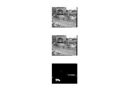
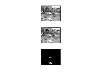
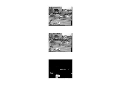
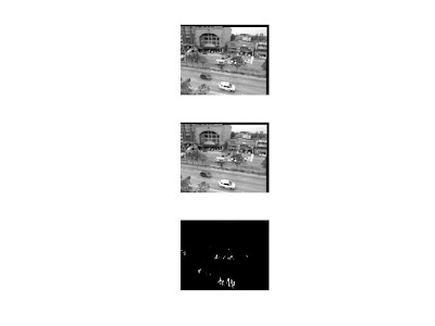
these operations are performed on a stabilized video sequence done by SIFT. and basic background subtraction.

se1 = strel('square',11) % 11-by-11 square
se2 = strel('line',10,45) % line, length 10, angle 45 degrees
se3 = strel('disk',15) % disk, radius 15
se4 = strel('ball',15,5) % ball, radius 15, height 5


sedisk = strel('square',10);
fg = imclose(fg, sedisk);


sedisk = strel('line',10,90);
fg = imclose(fg, sedisk);

sedisk = strel('line',15,5);
fg = imclose(fg, sedisk);


sedisk = strel('disk',10);
fg = imclose(fg, sedisk);


Deciding on the morphological structure is much harder than deciding on the threshold of background subtraction

High complexity background subtraction using mixture of guassian

The mean u of each Gaussian function, can be thought of as an educated guess of the pixel value in the next frame—we assume here that pixels are usually background. The weight and standard deviations of each component are measures of our confidence in that guess (higher weight & lower σ = higher confidence). There are typically 3-5 Gaussian components per pixel—the number typically depending on memory limitations.

In the image, the left images show the startup where all pixels are assumed to be background.through out the course of the video the background will be constructed. in contrast to median filter where it estimates and clears up the background.

Code:

% ----------------------- frame size variables -----------------------

fr = source(1).cdata; % read in 1st frame as background frame
fr_bw = rgb2gray(fr); % convert background to greyscale
fr_size = size(fr);
width = fr_size(2);
height = fr_size(1);
fg = zeros(height, width);
bg_bw = zeros(height, width);

% --------------------- mog variables -----------------------------------

C = 3; % number of gaussian components (typically 3-5)
M = 3; % number of background components
D = 2.5; % positive deviation threshold
alpha = 0.01; % learning rate (between 0 and 1) (from paper 0.01)
thresh = 0.25; % foreground threshold (0.25 or 0.75 in paper)
sd_init = 6; % initial standard deviation (for new components) var = 36 in paper
w = zeros(height,width,C); % initialize weights array
mean = zeros(height,width,C); % pixel means
sd = zeros(height,width,C); % pixel standard deviations
u_diff = zeros(height,width,C); % difference of each pixel from mean
p = alpha/(1/C); % initial p variable (used to update mean and sd)
rank = zeros(1,C); % rank of components (w/sd)


% --------------------- initialize component means and weights -----------

pixel_depth = 8; % 8-bit resolution
pixel_range = 2^pixel_depth -1; % pixel range (# of possible values)

for i=1:height
for j=1:width
for k=1:C

mean(i,j,k) = rand*pixel_range; % means random (0-255)
w(i,j,k) = 1/C; % weights uniformly dist
sd(i,j,k) = sd_init; % initialize to sd_init

end
end
end

%--------------------- process frames -----------------------------------

for n = 1:length(source)

fr = source(n).cdata; % read in frame
fr_bw = rgb2gray(fr); % convert frame to grayscale

% calculate difference of pixel values from mean
for m=1:C
u_diff(:,:,m) = abs(double(fr_bw) - double(mean(:,:,m)));
end

% update gaussian components for each pixel
for i=1:height
for j=1:width

match = 0;
for k=1:C
if (abs(u_diff(i,j,k)) <= D*sd(i,j,k)) % pixel matches component

match = 1; % variable to signal component match

% update weights, mean, sd, p
w(i,j,k) = (1-alpha)*w(i,j,k) + alpha;
p = alpha/w(i,j,k);
mean(i,j,k) = (1-p)*mean(i,j,k) + p*double(fr_bw(i,j));
sd(i,j,k) = sqrt((1-p)*(sd(i,j,k)^2) + p*((double(fr_bw(i,j)) - mean(i,j,k)))^2);
else % pixel doesn't match component
w(i,j,k) = (1-alpha)*w(i,j,k); % weight slighly decreases

end
end

w(i,j,:) = w(i,j,:)./sum(w(i,j,:));

bg_bw(i,j)=0;
for k=1:C
bg_bw(i,j) = bg_bw(i,j)+ mean(i,j,k)*w(i,j,k);
end

% if no components match, create new component
if (match == 0)
[min_w, min_w_index] = min(w(i,j,:));
mean(i,j,min_w_index) = double(fr_bw(i,j));
sd(i,j,min_w_index) = sd_init;
end

rank = w(i,j,:)./sd(i,j,:); % calculate component rank
rank_ind = [1:1:C];

% sort rank values
for k=2:C
for m=1:(k-1)

if (rank(:,:,k) > rank(:,:,m))
% swap max values
rank_temp = rank(:,:,m);
rank(:,:,m) = rank(:,:,k);
rank(:,:,k) = rank_temp;

% swap max index values
rank_ind_temp = rank_ind(m);
rank_ind(m) = rank_ind(k);
rank_ind(k) = rank_ind_temp;

end
end
end

% calculate foreground
match = 0;
k=1;

fg(i,j) = 0;
while ((match == 0)&&(k<=M))

if (w(i,j,rank_ind(k)) >= thresh)
if (abs(u_diff(i,j,rank_ind(k))) <= D*sd(i,j,rank_ind(k)))
fg(i,j) = 0;
match = 1;
else
fg(i,j) = fr_bw(i,j);
end
end
k = k+1;
end
end
end

figure(1),subplot(3,1,1),imshow(fr)
subplot(3,1,2),imshow(uint8(bg_bw))
subplot(3,1,3),imshow(uint8(fg))
end

medium complexity background subtraction using approximate median

In this method the previous N frames of video are buffered, and the background is calculated as the median of buffered frames. The problem is the background is cleared of all objects after few frames to show a cleared background.

Median filtering has been shown to be very robust and to have performance comparable to higher complexity methods. However, storing and processing many frames of video (as is often required to track slower moving objects) requires an often prohibitively large amount of memory. This can be alleviated somewhat by storing and processing frames at a rate lower than the frame rate— thereby lowering storage and computation requirements at the expense of a slower adapting background.

The approximate median method works as such: if a pixel in the current frame has a value larger than the corresponding background pixel, the background pixel is incremented by 1. Likewise, if the current pixel is less than the background pixel, the background is decremented by one. In this way, the background eventually converges to an estimate where half the input pixels are greater than the background, and half are less than the background—approximately the median (convergence time will vary based on frame rate and amount movement in the scene.)




for i = 2:length(source)

fr = source(i).cdata;
fr_bw = rgb2gray(fr); % convert frame to grayscale

fr_diff = abs(double(fr_bw) - double(bg_bw)); % avoid negative overflow

for j=1:width
for k=1:height

if ((fr_diff(k,j) > thresh))
fg(k,j) = fr_bw(k,j);
else
fg(k,j) = 0;
end

if (fr_bw(k,j) > bg_bw(k,j))
bg_bw(k,j) = bg_bw(k,j) + 1;
elseif (fr_bw(k,j) <>
bg_bw(k,j) = bg_bw(k,j) - 1;
end

end
end

figure(1),subplot(3,1,1),imshow(fr)
subplot(3,1,2),imshow(uint8(bg_bw))
subplot(3,1,3),imshow(uint8(fg))
end

Low complexity background subtraction using frame difference method

Frame differencing, also known as temporal difference, uses the video frame at time t-1 as the background model for the frame at time t. This technique is sensitive to noise and
variations in illumination, and does not consider local consistency
properties of the change mask.
This method also fails to segment the non-background objects if they stop moving. Since it uses only a single previous frame, frame differencing may not be able to identify the interior
pixels of a large, uniformly-colored moving object. This is commonly known as the aperture problem.


a major flaw of this method is that for objects with uniformly distributed intensity values, the pixels are interpreted as part of the background. Another problem is that objects must be continuously moving. If an object stays still for more than a frame period (1/fps), it becomes part of the background.
This method does have two major advantages. One obvious advantage is the modest computational load. Another is that the background model is highly adaptive. Since the background is based solely on the previous frame, it can adapt to changes in the background faster than any other method (at 1/fps to be precise). As we'll see later on, the frame difference method subtracts out extraneous background noise (such as waving trees), much better than the more complex approximate median and mixture of Gaussians methods.
A challenge with this method is determining the threshold value.

The video is a result of stabilization using SIFT features.

Code:

clear all;close all;clc;
source = aviread('stabilized');
thresh = 40;
bg = source(1).cdata; % read in 1st frame as background frame
bg_bw = rgb2gray(bg); % convert background to greyscale
% ----------------------- set frame size variables -----------------------
fr_size = size(bg);
width = fr_size(2);
height = fr_size(1);
fg = zeros(height, width);
% --------------------- process frames -----------------------------------
for i = 2:length(source)
fr = source(i).cdata; % read in frame
fr_bw = rgb2gray(fr); % convert frame to grayscale
fr_diff = abs(double(fr_bw) - double(bg_bw));
for j=1:width
for k=1:height
if ((fr_diff(k,j) > thresh))
fg(k,j) = fr_bw(k,j);
else
fg(k,j) = 0;
end
end
end
bg_bw = fr_bw;
figure(1),subplot(3,1,1),imshow(fr)
subplot(3,1,2),imshow(fr_bw)
subplot(3,1,3),imshow(uint8(fg))
end