IMAGE WARPING and MOSAICING

the process of combining multiple photographic images with overlapping fields of view to produce a segmented panorama or high-resolution image. Commonly performed through the use of computer software, most approaches to image stitching require nearly exact overlaps between images and identical exposures to produce seamless results.

My Steps

1. Convert the video into Frames and then into Images
   
2. using SIFT get pairs of corresponding points taken from the two images
3. Recover homographies of each Image
4. Warp the images using the homography
5. Blend images into a mosaic using weighted average
   
6. View the Results

a One minute video is 60*30 = 1800 images. Will reduce for speed.

function [mos_img]=mosaic(filename)
% creates a mosaic image from a movie
% assuming translation only between frames



warning off MATLAB:mir_warning_variable_used_as_function;

% using global names to cache frames in memory
% performance boosting
global Nframes;
global AviName;

AviName = filename;
[h, w, Nframes] = avi_size(AviName);

% relative displacements
d = zeros(2,Nframes);

RefFrame = GetImage(1);

% align every two consequent frames
for ii=2:Nframes

    % read a frame
    Frame = GetImage(ii);

    d(:,ii) = align(RefFrame, Frame, d(:,ii-1));

    % current frame is next one's reference
    RefFrame = Frame;
end

% cumulative displacement relative to first frame
D = cumsum(d,2);

% minimal
Minimum = min(D,[],2);
%maximal
Maximum = max(D,[],2);

% minimal displacement is one
D = D - Minimum*ones(1,Nframes)+1;

% create an empty mosaic (compute the bounding box)
mos_img = zeros([w, h]+ceil(Maximum'-Minimum'))';
[bm bn] = size(mos_img);
% creates weights
weights = zeros(bm,bn);

% shfoch everything into the mosaic
for ii=1:Nframes
    % read a frame
    Frame = GetImage(ii);

    tmpF(1:(h+1),1:(w+1)) = 0;
    tmpF(2:h+1,2:w+1) = Frame;
    intD = floor(D(:,ii));
    wF = warp(tmpF, (D(:,ii)-intD));
    wF(find(isnan(wF))) = 0;

    % mask
    m = zeros(size(tmpF));
    m(2:h+1,2:w+1) = 1;
    wm = warp(m, (D(:,ii)-intD));
    wm(find(isnan(wm))) = 0;

    [A B] = GetPosArray(bm, h, bn, w, intD);
    mos_img(A, B) = mos_img(A, B) + wF;
    weights(A, B) = weights(A, B) + wm;

end

weights = weights + (weights == 0); % in order to avoid zero division
mos_img = mos_img./weights;



function [A, B] = GetPosArray(bm, h, bn, w, intD)
% Gets an array, where to put the image.
% bm, bn - the total image's size
% h, w - single frame's size
% intD - the integer displacement.
A = bm - h + 1 - intD(2): bm - intD(2) + 1;
B = bn - w + 1- intD(1): bn - intD(1) + 1;



function image = GetImage(index)
% Gets the image data in the correct form (Double, greyscale).
% using chached frames to boost performance

% caching BUFFER_SIZE images at each access to the avi file
BUFFER_SIZE = 40;
persistent CurrentBlock M;
global AviName Nframes;

if (isempty(CurrentBlock))
    CurrentBlock = -1;
end;

% zindex to start from zero rather than one.
zindex = index - 1;

if (floor(zindex / BUFFER_SIZE) ~= CurrentBlock)
    CurrentBlock = zindex / BUFFER_SIZE;
    ReadTo = min((CurrentBlock+1)*BUFFER_SIZE, Nframes);
    M = aviread(AviName, (CurrentBlock*BUFFER_SIZE + 1):ReadTo);
end

localIndex = mod(zindex, BUFFER_SIZE) + 1;

%returning the right image in the correct format.
image = im2double(rgb2gray(M(localIndex).cdata ));



function [shift] = align(im1, im2, initial_shift)
% This function aligns im2 to im1 assuming an homography consist of shift only
% Input parameters
%   im1, im2 - images in double representation grey level range [0,1]
%
% The output parameters:
%   shift - a vector [dx, dy]' of displacement



% initial guess for displacement
shift = [0, 0]';
if (nargin == 3)
    shift = initial_shift;
end;

% global parameters
ITER_EPS = 0.001;
PYRAMID_DEPTH = 5;
ITERATIONS_PER_LEVEL = 5;
FILTER_PARAM = 0.4;         % parameter for gaussian pyramid

% Creating pyramids for both images.
F = gaussian_pyramid(im1, PYRAMID_DEPTH, FILTER_PARAM);
G = gaussian_pyramid(im2, PYRAMID_DEPTH, FILTER_PARAM);

% Allowing initial shift - scale it to fit pyramid level
shift = shift ./ (2^(PYRAMID_DEPTH+1));

% work coarse to fine in pyramids
for ii = PYRAMID_DEPTH : -1 : 1 %PYRAMID_DEPTH
    clear warped_im2;    % we are about to change its dimensionality

    shift = 2 * shift;   % compensate the scale factor between pyramid levels.

    % compute the gradient once per pyramid level
    [Fx Fy] = gradient(F{ii});

    % although we can re-calculate it according to overlapping zone
    % it is negligible thus we save computation by doing it once per level
    tmp = sum(Fx(:).*Fy(:));
    A = inv( [ sum(Fx(:).^2) tmp ; tmp sum(Fy(:).^2) ] );

    % iterate per pyramid level
    for jj = 1 : ITERATIONS_PER_LEVEL
        % always warp original image by accumulated shift, avoid over
        % blurring
        warped_im2 = warp(G{ii}, shift);

        % mask to rule out boundary (NaN values)
        mask = isnan(warped_im2);
        warped_im2(find(mask)) = 0;
        mask = 1-mask;

        % difference image - ignore parts that are not overlapping
        diff = ( F{ii}(:)-warped_im2(:) ).*mask(:);

        % Solve and update shift;
        tmpshift =  A*[sum(diff.*Fx(:)) ; sum(diff.*Fy(:))] ;
        shift = shift + tmpshift;
        if (abs(tmpshift) < ITER_EPS)
            break;
        end;
    end;
end;

% wrapping an image with shift using bilinear interpolation
function [warped] = warp(image, shift)
[x y] = size(image);
[X Y] = meshgrid(1:y,1:x); % Behold!!!
warped = interp2(image, X+shift(1), Y+shift(2), 'linear');


function [G] = gaussian_pyramid(image, n, a)
% compute n gaussian pyramid of an image
% a - filter parameter

G = cell(n,1);
G{1} = image;
for ii=1:n-1
    % use tmp variable to comply with varying size of image through down sampling
    G{ii+1}=gaussian_pyramid_one_stage(G{ii}, a);
end


function [G]=gaussian_pyramid_one_stage(im, a)
% compute one stage of a gaussian pyramid of an image
% a is the filter parameter

[m n]=size(im);

% construct the filter
filterKernel = [0.25 - (a/2), 0.25, a, 0.25, 0.25-(a/2)];
h = filterKernel'*filterKernel;

% filter the image, i.e. blur it with the gaussian, replicate to overcome
% boundary conditions
filt = imfilter(im, h, 'replicate');

% down sample
G = filt(1:2:m,1:2:n);

Detecting Corners using CornerMetric

The cornermetric function identifies corners in an image. The two algorithms employed by the function—the Harris corner detection method (the default) and Shi and Tomasi's minimum eigenvalue method—both use the eigenvalues of the summation of the squared difference matrix (SSD). The eigenvalues of an SSD matrix represent the differences between the surroundings of a pixel and the surroundings of its neighbors. The larger the difference between the surroundings of a pixel and those of its neighbors, the larger the eigenvalues. The larger the eigenvalues, the more likely a pixel is at a corner.


I = imread('1.jpg');
C = cornermetric(I, 'SensitivityFactor', 0.01);
imshow(I);
[y, x] = find(corner_peaks);
hold on
plot(x, y, '.', 'Color', 'y')
hold off

Video stabilization - using sift

first video shows Original video with Unwanted camera shake
second video shows result of video without camera shake




Buit in matlab function:
CP2TFORM Infer spatial transformation from control point pairs.
CP2TFORM takes pairs of control points and uses them to infer a
spatial transformation.


CP2TFORM requires a minimum number of control point pairs to infer a
% TFORM structure of each TRANSFORMTYPE:
%
% TRANSFORMTYPE MINIMUM NUMBER OF PAIRS
% ------------- -----------------------
% 'nonreflective similarity' 2
% 'similarity' 3
% 'affine' 3
% 'projective' 4


http://www.mathworks.com/access/helpdesk/help/toolbox/images/cp2tform.html

given a set of points "inp" in the first image
another set of points "outp" in another image
recompute the change in the projected points

Code:

% compute the similarity transformation
tt = cp2tform(inp, outp, 'linear conformal');
L = tt.tdata.T;
scale = sqrt(L(1,1)^2 + L(1,2)^2);
L(:,1:2) = L(:,1:2)/scale;
% sum the transforms up
T = T + L;
end

% get the average transformation
T = T/count;

% warping by backprojection.
% inv(T) is the transform from target back to the original image
T = inv(T);

width = size(im, 2);
height = size(im, 1);
% x and y are coordinates on the warped image
[x,y] = meshgrid(1:width, 1:height);
nxy = [x(:), y(:), ones(length(x(:)), 1)] * T;
% newx and newx are corresponding point coordinates in the original image
newx = reshape(nxy(:,1), height, width);
newy = reshape(nxy(:,2), height, width);

Math:

For an ‘affine’ transformation, the parametric motion can be described by the following formulas:

u(x,y) = a1x + a2y + a3
v(x,y) = a4x + a5y + a6

In this case there are six unknowns namely a1 –> a6 . In order to solve for these unknowns we must expand matrices to this form:







Since u1 –> u3 and v1 –> v3 can be easily calculated using the 3 pairs of points from each image and (x1 –> x3 , y1 –> y3) are already known, a1 –> a6 can be solved by using the formula v = (AT*A)-1 * AT b where (AT*A)-1 is defined as the pseudo inverse of A. With these new values imtransform() can modify the first image to correspond with the second image. xdata and ydata are variables describing the offset between the static image and transformed image, while trans is the scaled and sheared transformed image.


For a projective transformation: [up vp wp] = [x y w] T, where

u = up / wp
v = vp / wp.


T is a 3-by-3 matrix, where all nine elements can be different.

T = [ A D G
B E H
C F I]


The above matrix equation is equivalent to these two expressions:

u = (Ax + By + C) / (Gx + Hy + 1)
v = (Dx + Ey + F) / (Gx + Hy + 1)

Summary:

For a projective transformation:

u = (Ax + By + C)/(Gx + Hy + I)
v = (Dx + Ey + F)/(Gx + Hy + I)

Assume I = 1, multiply both equations, by denominator:

u = [x y 1 0 0 0 -ux -uy] * [A B C D E F G H]'
v = [0 0 0 x y 1 -vx -vy] * [A B C D E F G H]'

With 4 or more correspondence points we can combine the u equations and
the v equations for one linear system to solve for [A B C D E F G H]:

[ u1 ] = [ x1 y1 1 0 0 0 -u1*x1 -u1*y1 ] * [A]
[ u2 ] = [ x2 y2 1 0 0 0 -u2*x2 -u2*y2 ] [B]
[ u3 ] = [ x3 y3 1 0 0 0 -u3*x3 -u3*y3 ] [C]
[ u1 ] = [ x4 y4 1 0 0 0 -u4*x4 -u4*y4 ] [D]
[ ... ] [ ... ] [E]
[ un ] = [ xn yn 1 0 0 0 -un*xn -un*yn ] [F]
[ v1 ] = [ 0 0 0 x1 y1 1 -v1*x1 -v1*y1 ] [G]
[ v2 ] = [ 0 0 0 x2 y2 1 -v2*x2 -v2*y2 ] [H]
[ v3 ] = [ 0 0 0 x3 y3 1 -v3*x3 -v3*y3 ]
[ v4 ] = [ 0 0 0 x4 y4 1 -v4*x4 -v4*y4 ]
[ ... ] [ ... ]
[ vn ] = [ 0 0 0 xn yn 1 -vn*xn -vn*yn ]

Or rewriting the above matrix equation:
U = X * Tvec, where Tvec = [A B C D E F G H]'
so Tvec = X\U.

2D homography using SIFT features

Finding Global motion estimation for 2 images.
Using SIFT, Much more point correspondences. Faster than RANSAC. can be used in real time videos.

Sift Code used is from Lowe's implementation.
Source: http://www.cs.ubc.ca/~lowe/keypoints/

TO DO:
use Video Clip for Matches

Pure Matlab Code:

function num = match(image1, image2)

% Find SIFT keypoints for each image
[im1, des1, loc1] = sift(image1);
[im2, des2, loc2] = sift(image2);

% For efficiency in Matlab, it is cheaper to compute dot products between
% unit vectors rather than Euclidean distances. Note that the ratio of
% angles (acos of dot products of unit vectors) is a close approximation
% to the ratio of Euclidean distances for small angles.
%
% distRatio: Only keep matches in which the ratio of vector angles from the
% nearest to second nearest neighbor is less than distRatio.
distRatio = 0.6;

% For each descriptor in the first image, select its match to second image.
des2t = des2'; % Precompute matrix transpose
for i = 1 : size(des1,1)
dotprods = des1(i,:) * des2t; % Computes vector of dot products
[vals,indx] = sort(acos(dotprods)); % Take inverse cosine and sort results

% Check if nearest neighbor has angle less than distRatio times 2nd.
if (vals(1) < im3 =" appendimages(im1,im2);" cols1 =" size(im1,2);" i =" 1:"> 0)
line([loc1(i,2) loc2(match(i),2)+cols1], ...
[loc1(i,1) loc2(match(i),1)], 'Color', 'c');
end
end
hold off;
num = sum(match > 0);
fprintf('Found %d matches.\n', num);

Computation of 2D homography using RANSAC

Initial Images:

The first step of the algorithm is to compute interest points in each image. We are then faced with a "chicken and egg" problem: once the correspondence between the interest points is established the homography can be computed; conversely, given the homography the correspondence between the interest points can easily be established. This problem is resolved by using robust estimation, here RANSAC, as a "search engine".
The idea is first to obtain by some means a set of putative point correspondences. It is expected that a proportion of these correspondences will in fact be mismatches. RANSAC is designed to deal with exactly this situation - estimate the homography and also a set of inliers consistent with this estimate (the true correspondences), and outliers (the mismatches).



Initial Code:

thresh = 500; % Harris corner threshold
nonmaxrad = 3; % Non-maximal suppression radius
dmax = 100;
w = 11; % Window size for correlation matching

im1 = rgb2gray(imread('use1.jpg'));
im2 = rgb2gray(imread('use2.jpg'));

% Find Harris corners in image1 and image2
[cim1, r1, c1] = harris(im1, 1, thresh, 3);
show(im1,1), hold on, plot(c1,r1,'r+');

[cim2, r2, c2] = harris(im2, 1, thresh, 3);
show(im2,2), hold on, plot(c2,r2,'r+');

drawnow

tic
[m1,m2] = matchbycorrelation(im1, [r1';c1'], im2, [r2';c2'], w, dmax);
toc
% Display putative matches
show(im1,3), set(3,'name','Putative matches'), hold on
for n = 1:length(m1);
line([m1(2,n) m2(2,n)], [m1(1,n) m2(1,n)])
end

% Assemble homogeneous feature coordinates for fitting of the
% homography matrix, note that [x,y] corresponds to [col, row]
x1 = [m1(2,:); m1(1,:); ones(1,length(m1))];
x2 = [m2(2,:); m2(1,:); ones(1,length(m1))];

t = .001; % Distance threshold for deciding outliers
[H, inliers] = ransacfithomography_vgg(x1, x2, t);

fprintf('Number of inliers was %d (%d%%) \n', ...
length(inliers),round(100*length(inliers)/length(m1)))
fprintf('Number of putative matches was %d \n', length(m1))

% Display both images overlayed with inlying matched feature points
show(double(im1)+double(im2),4), set(4,'name','Inlying matches'), hold on
plot(m1(2,inliers),m1(1,inliers),'r+');
plot(m2(2,inliers),m2(1,inliers),'g+');

% Step through each matched pair of points and display the
% line linking the points on the overlayed images.

for n = inliers
line([m1(2,n) m2(2,n)], [m1(1,n) m2(1,n)],'color',[0 0 1])
end

return

Feature detection using Scale-invariant feature transform (SIFT)

an algorithm in computer vision to detect and describe local features in images. The algorithm was published by David Lowe in 1999.

images and details from (based on my understanding):
Lowe, David G. “Distinctive Image Features from Scale­ Invariant Keypoints”. International Journal of Computer Vision, 60, 2 (2004)

Applications include object recognition, robotic mapping and navigation, image stitching, 3D modeling, gesture recognition, video tracking, and match moving.

Source: http://en.wikipedia.org/wiki/Scale-invariant_feature_transform


Results
TO DO: publish source code (Pure matlab)
Leave a comment for the source code


% Computation of the maximum number of levels:
Lmax = floor(min(log(2*size(img)/12)/log(scl)));

%build image pyramid and difference of gaussians filter response pyramid
[pyr,imp] = build_pyramid(img,Lmax,scl);
%get the feature points
pts = find_features(pyr,img,scl,thresh,radius,radius2,disp_flag,1);

%classify points and create sub-pixel and sub-scale adjustments
[features,keys] = refine_features(img,pyr,scl,imp,pts,radius3,min_sep,edgeratio);

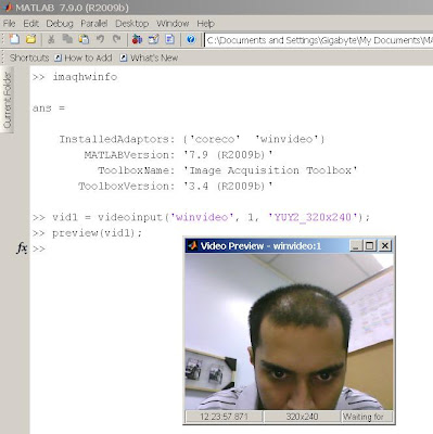
use live video to Capture Images for processing

Prereq: Matlab 7.9 R2009b

Check to see if the toolbox is installed before checking for the adapters.

after checking the adapters select any and type the commands to have a preview.

TO DO: process the live video

Corner Detection using Harris

Harris and Stephens improved upon Moravec's corner detector by considering the differential of the corner score with respect to direction directly, instead of using shifted patches. (This corner score is often referred to as autocorrelation, since the term is used in the paper in which this detector is described. However, the mathematics in the paper clearly indicate that the sum of squared differences is used.)

C. Harris and M. Stephens (1988). "A combined corner and edge detector" (PDF). Proceedings of the 4th Alvey Vision Conference. pp. 147--151. http://www.csse.uwa.edu.au/~pk/research/matlabfns/Spatial/Docs/Harris/A_Combined_Corner_and_Edge_Detector.pdf.

How does it work?
The first step in Harris is to compute a corner response function. Harris uses a series of filters that are considered the most important steps to find a corner. These kernels are:

• A presmoothing filter pfilt = {0.223755f,0.552490f,0.223755f};
• a gradient filter gfilt = {0.453014f,0.0f,-0.453014f};
• a Blur Filter bfilt = {0.01563f,0.09375f,0.234375f,0.3125f, 4 0.234375f,0.09375f,0.01563f};

The combination of these filters and few parameters are what make Harris successful in finding corners. The parameters are as followed::

• Steering parameter 0.04 - 0.06 (0.05 default)
• Response threshold 10K - 1M (default 25,000)
• neighborhood radius 10 pixels

clear all
close all
clc;

disp('Harris Corner detection Purposes Only....');

fin = 'smallVersion2.avi'; %input File name to be changed
fout = 'movie2.avi'; %output File name to be changed

%get the File info
fileinfo = aviinfo(fin);
%get the number of Frames
nframes = fileinfo.NumFrames;

aviobj = avifile(fout, 'compression', 'none', 'fps',fileinfo.FramesPerSecond);

for i = 1:nframes %You may need to limit the nFrames, may result in a large file size
%Read frames from input video
mov_in = aviread(fin,i);
im_in = frame2im(mov_in);

%Do processing on each frame of the video

im = rgb2gray(im_in);
% Find Harris corners in image1 and image2
if ~isa(im,'double')
im = double(im);
end

subpixel = nargout == 5;

dx = [-1 0 1; -1 0 1; -1 0 1]; % Derivative masks
dy = dx';

Ix = conv2(im, dx, 'same'); % Image derivatives
Iy = conv2(im, dy, 'same');

% Generate Gaussian filter of size 6*sigma (+/- 3sigma) and of
% minimum size 1x1.
sigma =1;
g = fspecial('gaussian',max(1,fix(6*sigma)), sigma);

Ix2 = conv2(Ix.^2, g, 'same'); % Smoothed squared image derivatives
Iy2 = conv2(Iy.^2, g, 'same');
Ixy = conv2(Ix.*Iy, g, 'same');
k = 0.04;
cim = (Ix2.*Iy2 - Ixy.^2) - k*(Ix2 + Iy2).^2; % Original Harris measure.


if nargin > 2 % We should perform nonmaximal suppression and threshold

if subpixel
[r,c,rsubp,csubp] = nonmaxsuppts(cim, 1, 10000, im);
else
[r,c] = nonmaxsuppts(cim, 1, 10000, im);
end
end


show(im,1), hold on, plot(c,r,'r+');
drawnow


%Write frames to output video
%frm = im2frame(im_out);
%aviobj = addframe(aviobj,frm);

%i %Just to display frame number you can ommit
end;

%Don't forget to close output file
aviobj = close(aviobj);
return;




function [r,c, rsubp, csubp] = nonmaxsuppts(cim, radius, thresh, im)

subPixel = nargout == 4; % We want sub-pixel locations
[rows,cols] = size(cim);

% Extract local maxima by performing a grey scale morphological
% dilation and then finding points in the corner strength image that
% match the dilated image and are also greater than the threshold.

sze = 2*radius+1; % Size of dilation mask.
mx = ordfilt2(cim,sze^2,ones(sze)); % Grey-scale dilate.

% Make mask to exclude points within radius of the image boundary.
bordermask = zeros(size(cim));
bordermask(radius+1:end-radius, radius+1:end-radius) = 1;

% Find maxima, threshold, and apply bordermask
cimmx = (cim==mx) & (cim>thresh) & bordermask;

[r,c] = find(cimmx); % Find row,col coords.


if subPixel % Compute local maxima to sub pixel accuracy
if ~isempty(r) % ...if we have some ponts to work with

ind = sub2ind(size(cim),r,c); % 1D indices of feature points
w = 1; % Width that we look out on each side of the feature
% point to fit a local parabola

% Indices of points above, below, left and right of feature point
indrminus1 = max(ind-w,1);
indrplus1 = min(ind+w,rows*cols);
indcminus1 = max(ind-w*rows,1);
indcplus1 = min(ind+w*rows,rows*cols);

% Solve for quadratic down rows
cy = cim(ind);
ay = (cim(indrminus1) + cim(indrplus1))/2 - cy;
by = ay + cy - cim(indrminus1);
rowshift = -w*by./(2*ay); % Maxima of quadradic

% Solve for quadratic across columns
cx = cim(ind);
ax = (cim(indcminus1) + cim(indcplus1))/2 - cx;
bx = ax + cx - cim(indcminus1);
colshift = -w*bx./(2*ax); % Maxima of quadradic

rsubp = r+rowshift; % Add subpixel corrections to original row
csubp = c+colshift; % and column coords.
else
rsubp = []; csubp = [];
end
end

if nargin==4 & ~isempty(r) % Overlay corners on supplied image.
figure(1), imshow(im,[]), hold on
if subPixel
plot(csubp,rsubp,'r+'), title('corners detected');
else
plot(c,r,'r+'), title('corners detected');
end
end

Moravec Corner Detection algorithm

This is one of the earliest corner detection algorithms and defines a corner to be a point with low self-similarity. The algorithm tests each pixel in the image to see if a corner is present, by considering how similar a patch centered on the pixel is to nearby, largely overlapping patches. The similarity is measured by taking the sum of squared differences (SSD) between the two patches. A lower number indicates more similarity.

If the pixel is in a region of uniform intensity, then the nearby patches will look similar. If the pixel is on an edge, then nearby patches in a direction perpendicular to the edge will look quite different, but nearby patches in a direction parallel to the edge will result only in a small change. If the pixel is on a feature with variation in all directions, then none of the nearby patches will look similar.

The corner strength is defined as the smallest SSD between the patch and its neighbors (horizontal, vertical and on the two diagonals). If this number is locally maximal, then a feature of interest is present.

As pointed out by Moravec, one of the main problems with this operator is that it is not isotropic: if an edge is present that is not in the direction of the neighbours, then it will not be detected as an interest point.

Denote the image intensity of a pixel at (x, y) by I(x, y).

Input: grayscale image, window size, threshold T
Output: map indicating position of each detected corner

1. For each pixel (x, y) in the image calculate the intensity variation from a shift (u, v) as:

where the shifts (u,v) considered are:
(1,0),(1,1),(0,1),(-1,1),(-1,0),(-1,-1),(0,-1),(1,-1)

2. Construct the cornerness map by calculating the cornerness measure C(x, y) for each pixel (x, y):

3. Threshold the interest map by setting all C(x, y) below a threshold T to zero.

4. Perform non-maximal suppression to find local maxima.

All non-zero points remaining in the cornerness map are corners.

Source:http://www.cim.mcgill.ca/~dparks/CornerDetector/mainMoravec.htm

Matlab Code:
% calculate moravec operator of an image
function [corner,ch,cv,cd1,cd2] = cornerMoravec(I,border)


hori = [1 -1];
vert = hori';
diag1 = [1 0; 0 -1];
diag2 = [0 1; -1 0];


average = ones(4,4); % average filter


conv_type='same';


h = conv2(I,hori,conv_type);
v = conv2(I,vert,conv_type);
d1 = conv2(I,diag1,conv_type);
d2 = conv2(I,diag2,conv_type);


c=zeros(size(I));
for i=1:prod(size(I))
c(i) = min([h(i)^2 v(i)^2 d1(i)^2 d2(i)^2]);
end


for i=2:size(I,1)-1
for j=2:size(I,2)-1


hh = sum(sum(abs(h(i-1:i+1,j-1:j+1)))); % 3x3 subimage
vv = sum(sum(abs(v(i-1:i+1,j-1:j+1)))); % 3x3 subimage
dd1 = sum(sum(abs(d1(i-1:i+1,j-1:j+1)))); % 3x3 subimage
dd2 = sum(sum(abs(d2(i-1:i+1,j-1:j+1)))); % 3x3 subimage


c(i,j) = min(hh,min(vv,min(dd1,dd2)));
ch(i,j) = hh;
cv(i,j) = vv;
cd1(i,j) = dd1;
cd2(i,j) = dd2;


end
end


corner=c;
corner=corner(border+1:end-border,border+1:end-border);
ch = ch(border+1:end-border,border+1:end-border);
cv = cv(border+1:end-border,border+1:end-border);
cd1 = cd1(border+1:end-border,border+1:end-border);
cd2 = cd2(border+1:end-border,border+1:end-border);
.